PeakLab v2 Documentation Contents            R2N Software Home            R2N Software Support

Filter Background MS Data

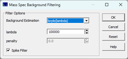
The Filter Background/Spikes in MS Data... in the MassSpec menu opens the following dialog to perform a background filtration of spikes and ionization noise. You must first import MS data using the MassSpec | Import MZML data... or the MassSpec | Import Agilent data.ms Data... option.



This uses the same pybaselines Whittaker routines that are used in the Baseline procedure. The procedure is computationally intensive and can require a minute or more to complete the filtration. You simply select the algorithm of choice and set the lambda, and penalty if the algorithm has a 'p' parameter, and check if you wish to have spikes filtered from the data, and click OK.

When the background is computed, it will consist of a large number of MS1 XICs each of which will be independently processed for a Whittaker baseline correction.

The Algorithm: High-Density Channel-by-Channel Baseline Subtraction

This procedure uses a high-density baseline subtraction engine designed to isolate and remove the continuous ionization background (often seen as chemical noise) inherent in high-resolution mass spectrometry (HRMS) data. Instead of treating the entire LC-MS or GC-MS run as a single 3D topographical map, this algorithm dissects the data into thousands of distinct, 1-dimensional Extracted Ion Chromatograms (XICs) and cleans each one individually.

Here is a breakdown of how the algorithm operates:

Data Dissection

When the raw data array is handed to the algorithm, it does not immediately start fitting.

Rounding and Grouping: It first rounds the high-resolution m/z values to integer values. This effectively bins the data into distinct nominal mass "channels" (e.g., all signals at m/z 204.01, 204.05, and 204.12 are temporarily treated as a single trace for m/z 204).

Masking: The script uses a unique_channels loop to iterate through every single nominal mass present in the run. For a typical HRMS dataset, this can result in thousands or even tens of thousands of individual XIC traces that must be processed independently.

The Pre-Filter: Time-Gap Despiking (Optional)

Before any mathematical fitting occurs on a given channel, the algorithm applies an optional "despiking" filter to remove ionization artifacts (often referred to in the script as "Green Starfield" artifacts).

It analyzes the time gaps between consecutive data points within the specific m/z trace.

If a point is completely isolated in time (meaning the time gap before and after it exceeds a calculated dynamic threshold, usually 3x the median gap), the algorithm flags it as an anomalous spike rather than a real chromatographic peak and forces its intensity to zero. This prevents massive single-point artifacts from distorting the subsequent baseline fit.

The Core Fitting Engine

Once a channel is isolated and despiked, the mathematical heavy lifting begins. The script utilizes the pybaselines Whittaker algorithms to perform the actual baseline estimation.

The user can select from over a dozen distinct algorithmic variations (e.g., arPLS, drPLS, asPLS, asLS), but they all share the same fundamental mathematical DNA: Whittaker Smoothing with Asymmetric Penalties.

The Balancing Act: The algorithm attempts to draw a baseline through the raw data by minimizing a specialized function. It balances two competing goals:

Fidelity: The baseline should stay as close to the data as possible.

Smoothness: The baseline should not be jagged; it must resist sharp changes (governed by the stiffness parameter, lambda).

The Asymmetric Weighting: Standard smoothing would just cut straight through the middle of the chromatographic peaks. To prevent this, these algorithms use asymmetric weighting (governed by the p parameter). During the iterative fitting loop, if a data point is above the current baseline estimate (suggesting it is a peak), it is given an extremely low weight. If a point is below the baseline, it is given a high weight. This forces the mathematical curve to rigidly anchor itself to the noise floor while "ignoring" the peaks rising above it.

The Iterative Matrix Math: Finding this perfect balance requires solving massive banded matrix equations (specifically, finding the inverse of pentadiagonal matrices). The algorithm guesses a baseline, calculates the asymmetric weights, solves the massive matrix to find a new baseline, recalculates the weights, and repeats this loop until the baseline stops moving (convergence).

The Subtraction and Clamping

Once the algorithm converges on the optimal baseline for that specific m/z channel, it executes the final cleanup. It subtracts the calculated baseline from the original raw data trace. Because mathematical baselines can sometimes dip slightly above the noise floor, the subtraction might result in negative intensities. The algorithm strictly clamps any negative values (or values less than 1.0) back to 0.0.

The cleaned trace is then injected back into the master data array, and the loop moves on to the next m/z channel.

Why is it so computationally heavy?

The sheer computational load comes from the nested multiplicative effect of the algorithm's architecture:

The Channel Multiplier: It does not solve one matrix for the file. If an LC-MS run has 2,000 unique nominal masses, the engine must spin up and execute 2,000 completely separate baseline analyses.

The Matrix Multiplier: For each of those 2,000 channels, the Whittaker algorithm requires solving a dense system of linear equations where the size of the matrix is determined by the number of scans in the run.

The Iteration Multiplier: Because the asymmetric weights must be updated dynamically, each channel cannot be solved in a single pass. It often requires 10 to 50 iterative loops of matrix inversions before a single channel converges.

The Filtered MZML File

PeakLab writes a new filtered MZML file containing only the filtered MS1 data to the same folder as the original data file. You must be certain that folder has write permission. It cannot be read only. The file will contain the same name, except that the algorithm is added in parentheses to the end of the file name. For example file.mzML would become file(drpls).mzML. When all of the backgrounds have been subtracted, you will see a plot of the filtered data:
 

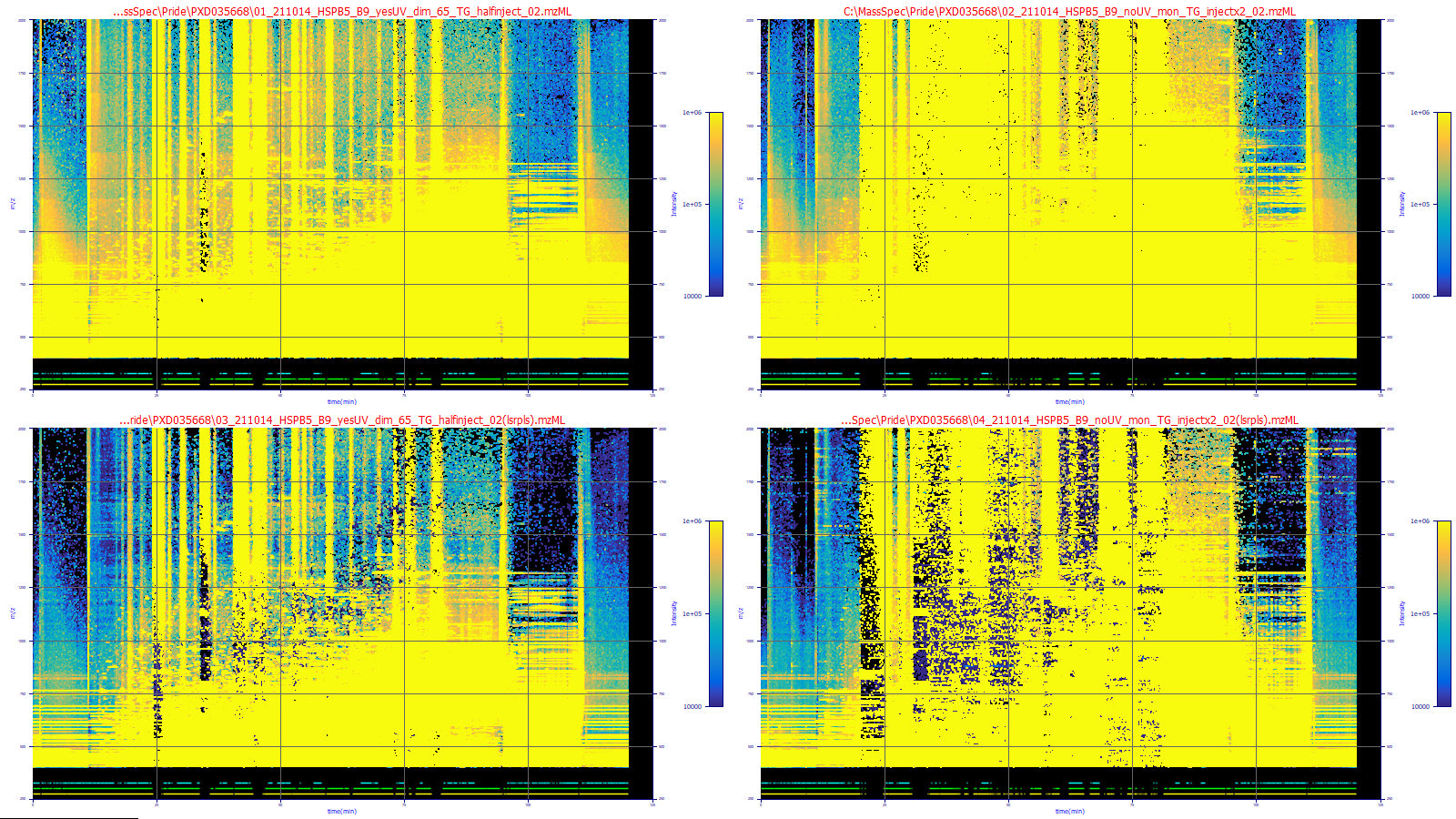
These plots were adjusted to highlight just the background (in blue). There are two sets in the plot, the filtered below the unfiltered. You will see that the filtered plots have a much better defined background. The first data set is a lower concentration, the second a much higher one. Both have a considerable measure of ionization noise.

Since the original files were likely MS1/MS2, very large, and unfiltered, you will likely want to load these smaller filtered MS1 files in any subsequent import of MS data. Once data have been filtered, these are the data which will be used in any further procedures until such time the data have been cleared or new MS data loaded.