PeakLab v1 Documentation Contents AIST Software Home AIST Software Support
White Paper: XPS Spectral Shapes
XPS Spectral Shapes
X-ray photoelectron spectroscopy (XPS) peaks, unlike many peaks in the spectral sciences, have an intrinsic asymmetry which makes modeling those shapes to a high measure of accuracy quite difficult. If the aim of the peak fitting is to recover the specific measure of Gaussian and Lorentzian character in the peak, the asymmetry must be removed in either a fitting procedure or in a Fourier preprocessing.

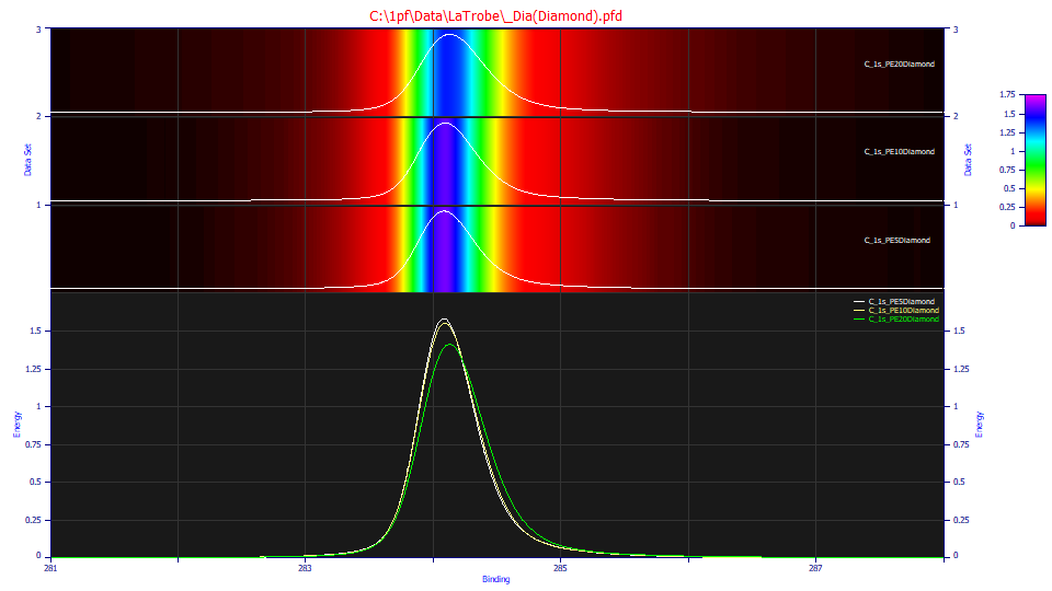
If the binding energies are shown in an increasing scale, the asymmetry in an XPS peak is right-shifted. The above XPS data us for a pure C peak in a diamond sample1. The three different peaks arise from 5, 10, and 20 eV pass energies. Note the highly-broadened tails in both the contours and in the peak shapes, and the rather appreciable asymmetry. While the 5 and 10 eV peaks are close in shape, the 20eV peak has a very different shape.
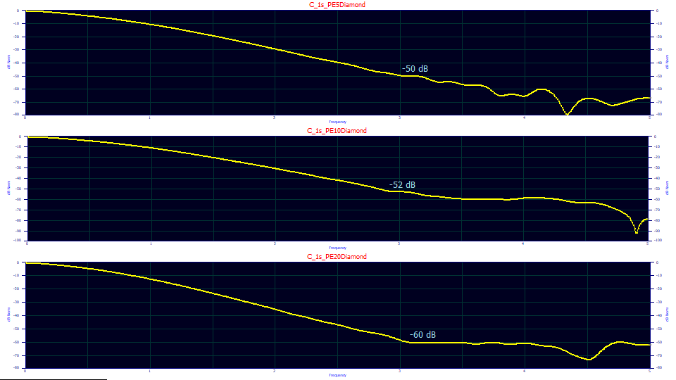
If the Fourier spectra of these data are plotted, the three different pass energies produce a higher S/N as the pass energy increases. If we use the first point of leveling to extract an estimated S/N, we see -50, -52, and -60 dB for the threshold where noise begins to appear. We would thus expect to see the best goodness of fit on the 20 eV PE analysis, and the least on the 5 eV.
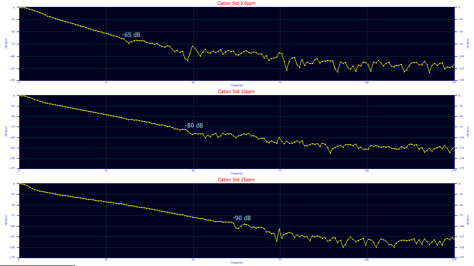
How does this compare with the chromatography peaks for which this <ge> IRF modeling was designed? The above Fourier data are for three different concentrations of a chromatographic peak. The S/N is approximately an order of magnitude stronger (20 db corresponds to 1 order of magnitude, or 1 additional digit of accuracy. If we see 2-4 ppm error in a near-perfect fit of the chromatography data, a realistic expectation for an XPS fit, based on S/N, might roughly be errors about 10x higher, or 20-40 ppm.
XPS IRF Functions
To model the asymmetry in an XPS peak, we can use any one of the chromatography IRFs, if the only aim is to mathematically and empirically model this distortion and remove it. Another option is to use a half-Voigt, which will characterize the measure of Gaussian and Lorentzian in the asymmetric distortion.
VoigtGL Model
The Voigt peak fitting the two widths directly with a0 as the peak area is defined as follows:
a0 = Area
a1 = Center (mode)
a2 = Gaussian Width (SD)
a3 = Lorentzian Width
We will begin with the measure to which an IRF is needed. If we fit a symmetric VoigtGL model (directly fits both the Gaussian and Lorentzian widths in the Voigt convolution), we see a fit error in the vicinity of 4200 ppm in all three data sets.
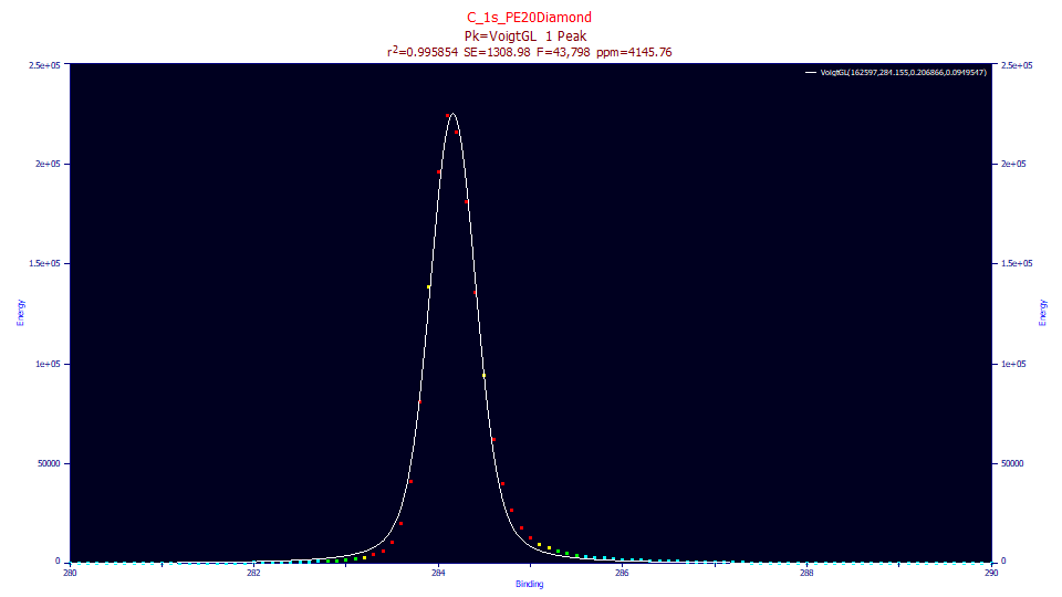
The above is the fit for the PE 20 eV data. The shape is clearly not fitted well.
VoigtGL<ge> Model
The chromatographic IRFs are mostly a sum of kinetic and/or one-sided probabilistic models.
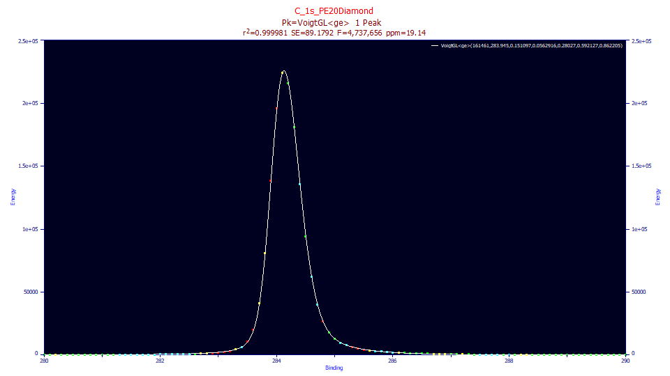
If the XPS diamond carbon peak is fitted to the VoigtGL<ge> model, the data are fitted to 29, 26, and 19 ppm error. Visually, the fit looks perfect, but in fairness it is impossible to visualize errors 100 ppm or smaller in an overall graph of a fit. The above plot is again for the PE 20 eV data. The <ge> IRF is a sum of a first-order exponential decay and a half-sided normal or Gaussian probabilistic function. There are three parameters in the <ge> IRF, a exponential time constant, the SD of the half-Gaussian SD, and an area fraction parameter that specifies how much of each of the two components are present:
|
|
Sum of Half-Gaussian and First Order Exponential
|
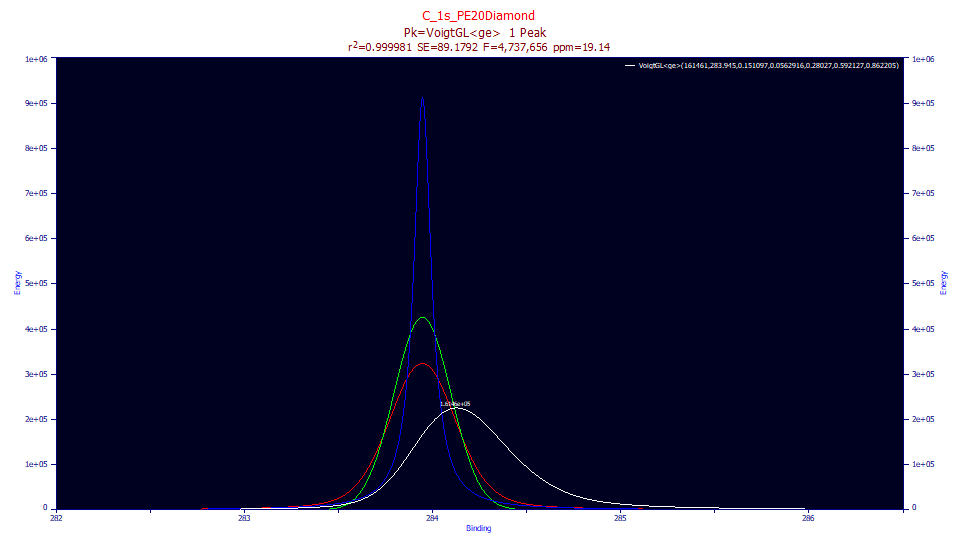
If we look at the deconvolutions this model makes possible, the white curve is the data as registered by the instrument. The red curve is the peak that would be seen if no asymmetry were present. This is the VoigtGL portion of the model with the <ge> IRF removed. The green curve if the Gaussian in the Voigt, and the blue curve is the Lorentzian. The blue Lorentzian and the green Gaussian components convolve to produce the red Voigt peak.
"C_1s_PE5Diamond"
Fitted Parameters
r2 Coef Det DF Adj r2 Fit Std Err F-value ppm uVar
0.99997082 0.99997045 65.0748274 3,107,201 29.1786708
Peak Type a0 a1 a2 a3 a4 a5 a6
1 VoigtGL<ge> 91008.2098 283.928281 0.12712134 0.06038603 0.23348227 0.40999399 0.78659231
"C_1s_PE10Diamond"
Fitted Parameters
r2 Coef Det DF Adj r2 Fit Std Err F-value ppm uVar
0.99997351 0.99997317 89.3195012 3,422,872 26.4877744
Peak Type a0 a1 a2 a3 a4 a5 a6
1 VoigtGL<ge> 1.3164e+05 283.926987 0.13387558 0.05582179 0.24854450 0.45714081 0.82411612
"C_1s_PE20Diamond"
Fitted Parameters
r2 Coef Det DF Adj r2 Fit Std Err F-value ppm uVar
0.99998086 0.99998062 89.1792268 4,737,656 19.1370840
Peak Type a0 a1 a2 a3 a4 a5 a6
1 VoigtGL<ge> 1.6146e+05 283.944946 0.15109741 0.05629157 0.28027001 0.59212691 0.86220481
The Gaussian peak width is a2, increasing from an SD width of 0.127 to 0.151 with increasing pass energy. The Lorentzian is a3, its width closer to constant between 0.055-0.060. The asymmetric distortion is represented as a mix of a half-Gaussian and first order kinetic. The a4 parameter is the width of the half-Gaussian, and its SD increases from 0.233 to 0.280 with increasing pass energy. The exponential tau or time constant also widens, from 0.410 to 0.592 as the pass energy setting is increased. The amount of half-Gaussian also increases, from 78.65% in the 5 eV sample to 86.2% on the 20 eV sample. If the aim of the fitting is to uncover the amount of Gaussian and Lorentzian absent the asymmetry, the IRF fitting exists only to recover the symmetric peak.
VoigtGL<v> Model
An alternative to an empirical IRF is to assume a portion of the original Voigt appears asymmetrically. If it is assumed that the Lorentzian and Gaussian components do not distribute in the same proportion as the core symmetric peak, we fit a <v> half-Voigt IRF which has its own separate Gaussian and Lorentzian widths. Note that this is not postulating a theoretical distortion associated with the asymmetry, only that a portion of each component of the Voigt will exist with a right-shifted, one-sided asymmetry. One thus estimates how much of the Gaussian distributes into the symmetric two-sided main peak, and how much into the IRF. Similarly, one is estimating how much of the Lorentzian distributes into the symmetric two-sided main Voigt peak, and how much belongs in the IRF describing the asymmetry.
|
|
Asymmetric Voigt (Gauss and Lorentz widths parameterization)
|
In the half-Voigt IRF, the Gaussian and Lorentzian components are convolved, just as is true in the symmetric Voigt describing the main peak. There are thus just two parameters since the two components convolve each another.
If we fit the Voigt<v> model to the diamond data, we see 87, 78, and 34 ppm errors. The errors are not quite as good, but may be more useful since the half-Voigt IRF may yield useful information with respect to how much of each of two different types of broadening enter into the peak's asymmetry.
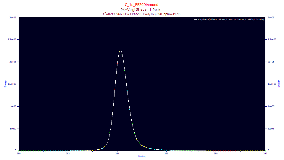
This is the 20 eV PE data for the Voigt<v> fit. It is a convolution of a Voigt with a half-Voigt, each of those being a convolution of a Gaussian and Lorentzian. It may sound complicated, but the Voigt, in its complex form is closed-form and no approximations or pseudo-Voigts are needed. The three data sets, fitted simultaneously to the Voigt<v> model, require less than a second in this fitting.
"C_1s_PE5Diamond"
Fitted Parameters
r2 Coef Det DF Adj r2 Fit Std Err F-value ppm uVar
0.99991235 0.99991138 112.683793 1,243,450 87.6516254
Peak Type a0 a1 a2 a3 a4 a5
1 VoigtGL<v> 92300.8644 283.924102 0.12427102 0.06173710 0.22311462 0.04974657
"C_1s_PE10Diamond"
Fitted Parameters
r2 Coef Det DF Adj r2 Fit Std Err F-value ppm uVar
0.99992237 0.99992152 152.766435 1,404,062 77.6258525
Peak Type a0 a1 a2 a3 a4 a5
1 VoigtGL<v> 1.3321e+05 283.924369 0.13184600 0.05705405 0.23608857 0.04671908
"C_1s_PE20Diamond"
Fitted Parameters
r2 Coef Det DF Adj r2 Fit Std Err F-value ppm uVar
0.99996555 0.99996517 119.546052 3,163,698 34.4521585
Peak Type a0 a1 a2 a3 a4 a5
1 VoigtGL<v> 1.6305e+05 283.945244 0.15161292 0.05617396 0.25882799 0.05192404
We see very nearly the same Gaussian SD and Lorentzian widths in the main peak. The IRF, however looks very different. The measure of Gaussian going into the half-Voigt is considerable, a width that increases slightly with pass energy from 0.223 to 0.259. Note that this is just under twice the width of the Gaussian seen in the deconvolved symmetric Voigt. The Lorentzian width in this half-Voigt is close to constant around 0.05. Note that this is only slightly smaller than the Lorentzian width that goes into the core Voigt peak. Note that the measure of asymmetric distortion is not insignificant, and the ratio of Gaussian to Lorentzian in this half-Voigt IRF is about twice that estimated for the core symmetric peak.
One can use the F-statistic to gauge whether one model is better from an information theoretic perspective than another. For the F-statistic to improve, each additional parameter in the model must make a substantive contribution to the over efficacy of the fitting. If we compare the F-statistic of the PE 20 fits of the GenHVL<ge> and GenHVL<v> model, we 4.74 million vs. 3.16 million. The additional IRF parameter in the GenHVL<ge> did offer a significant fitting improvement relative to the GenHVL<v> model.
Inspecting the half-Voigt IRF
The Gaussian or probabilistic component is present in both IRFs. In the <v> IRF, it is convolved with a Lorentzian, and in the <ge> IRF, it is used in a variable area sum with a first order exponential.
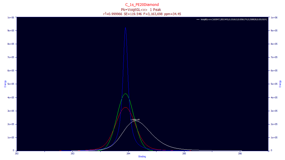
If we look at the deconvolutions in the Voigt<v> fit, we have the green Gaussian and blue Lorentzian convolving to form the red Voigt, the symmetric peak minus the IRF distortion.
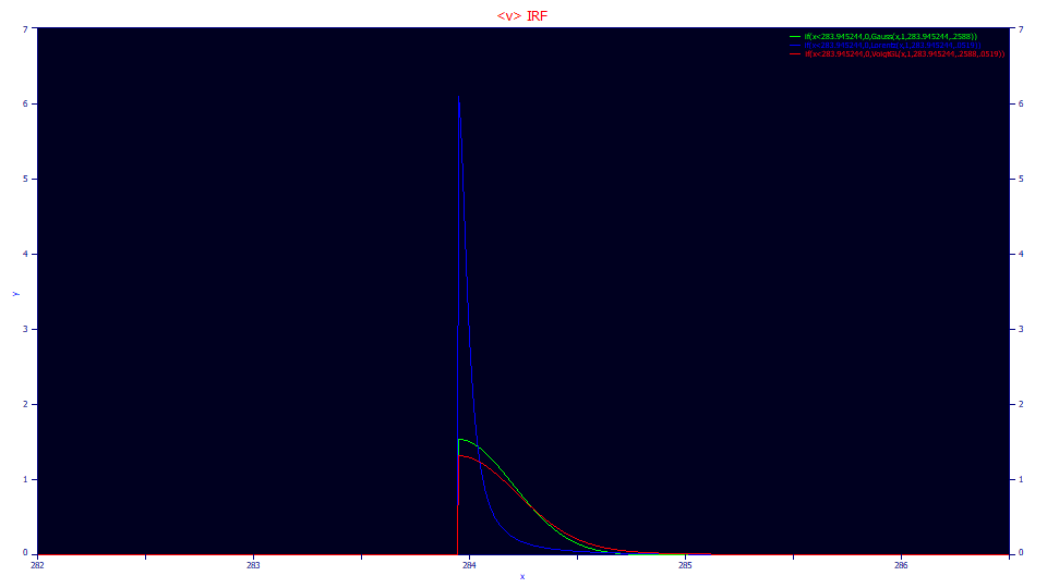
Above we plotted the half-Voigt <v> IRF on the same scale as the deconvolutions. The green is the Gaussian component of the IRF, the blue is the Lorentzian, and the red curve is the half-Voigt IRF that convolves the symmetric red Voigt peak in the first plot in order to produce the white observed asymmetric peak. By virtue of the Voigt parameters, it is possible to see the Lorentzian and Gaussian component of each.
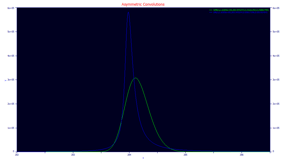
Since convolutions are commutative, we can look at the Voigt<v> model as Gauss ﺥ Lorentz ﺥ Half-Gauss ﺥ Half-Lorentz, we can use the fitted parameters to plot the Gauss ﺥ Half-Gauss and the Lorentz ﺥ Half-Lorentz convolutions in order to see the asymmetric Gaussian and asymmetric Lorentzian portions of the convolution. The first is a closed form half-Gaussian modified Gaussian, a GMG, and the second is a closed form half-Lorentzian modified Lorentzian, an LML. The GMG in green and the LML in blue also convolve to produce the white observed peak.
It may be useful to bear in mind that everything shown in the last three plots was derived from just six parameters in a Voigt<v> fit.
XPS Peak Comparisons
We will now perform the same fit with HDPE to the C peak. We will only use the 20 eV PE sample. We find one difference straightaway. Unlike the Diamond samples which required a half-Voigt IRF with its Lorentzian component to model the asymmetry, the HDPE sample cannot fit the half-Voigt IRFs to statistical significance. The Lorentzian component in the Voigt IRF iterates to zero. As such, only a half-Gaussian is needed in the IRF. The fits is as good, 26 ppm error.
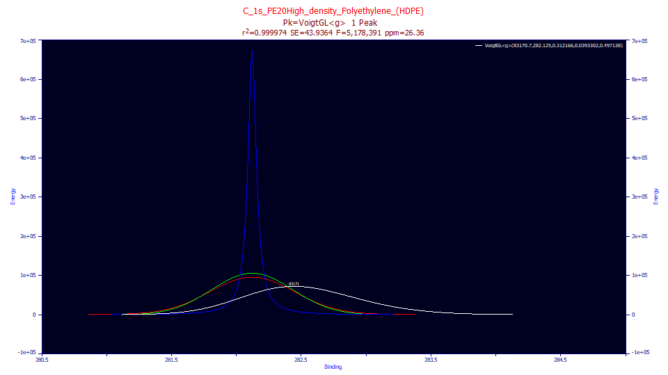
"C_1s_PE20High_density_Polyethylene_(HDPE)"
Fitted Parameters
r2 Coef Det DF Adj r2 Fit Std Err F-value ppm uVar
0.99997364 0.99997340 43.9364499 5,178,391 26.3588431
Peak Type a0 a1 a2 a3 a4
1 VoigtGL<g> 83170.6747 282.124808 0.31216573 0.03933018 0.49713843
Apart from the clear locational differences, 283.94 for the diamond and 282.12 for the HDPE, the blue Lorentzian looks sharper and indeed the Lorentzian width is smaller, 0.039 relative to the 0.056 of the diamond, but there is also the far more prominent matter of the Gaussian width of 0.312 being far larger than the 0.15 of the diamond. The Gaussian broadening now dominates to the point the main Voigt peak is far closer to the Gaussian (note the greater similarity of the red and green peaks). With respect to the IRF, the half-Gaussian SD value of 0.497 is also much higher than the 0.259 of the diamond.
In nonlinear modeling, one cannot definitively say that there is no Lorentzian component in the IRF, only that it is not possible to recover it via a fitting procedure. Here we might assume this inability to fit a Lorentzian in the IRF is due to the much greater measure of Gaussian broadening in both the main Voigt peak and in the IRF of the polymer.
1The diamond XPS data in this white paper were taken from the public domain XPSSurfA XPS data library, La Trobe University, Australia.