PeakLab v1 Documentation Contents            AIST Software Home            AIST Software Support

Baseline Optimization

Whittaker Algorithms

The Whittaker algorithms are numerous and varied, and each is designed to manage a specific type of baseline scenario.

arpls - Asymmetrically Reweighted Penalized Least Squares

Iteratively suppresses positive residuals (peaks) more than negative ones to estimate a smooth baseline without being biased by signal peaks.

lsrpls - Locally Symmetric Reweighted Penalized Least Squares

Applies symmetric weighting to penalized least squares, improving baseline fit in symmetric peak regions.

brpls - Bayesian Reweighted Penalized Least Squares

Uses Bayesian modeling to estimate peak proportions and reweight the baseline fit.

drpls - Doubly Reweighted Penalized Least Squares

Applies two layers of reweighting to better suppress peaks and noise during baseline estimation.

aspls - Adaptive Smoothness Penalized Least Squares

Dynamically adjusts the smoothing parameter across the signal to better handle variable baseline curvature.

iarpls - Improved Asymmetrically Reweighted Penalized Least Squares

Enhances arpls by refining the weighting scheme for better convergence and peak suppression.

psalsa - Peaked Signal's Asymmetric Least Squares Algorithm

Like asls but uses exponential decay weighting for values above the baseline, allowing better handling of noisy, peak-heavy data.

derpsalsa - Derivative Peak-Screening Asymmetric Least Squares Algorithm

Enhances psalsa by screening peaks using smoothed first and second derivatives before reweighting.

asls - Asymmetric Least Squares Smoothing

Classic baseline method that penalizes positive residuals more than negative ones to suppress peak.

iasls - Improved Asymmetric Least Squares Smoothing

Extends asls by incorporating both first and second derivatives of residuals.

airpls - Adaptive Iteratively Reweighted Penalized Least Squares

Iteratively updates weights based on residuals, adaptively suppressing peaks and improving convergence.

Whittaker Algorithm Optimization to Match Human Designed Baselines

Since it is difficult to determine which of these algorithms is most beneficial to your specific data and baseline, PeakLab offers an option where you can manually create your "perfect" baseline and then use a genetic differential evolution algorith to find the optimal settings for that specific training example.

This is invoked by the Optimize button in the Baseline procedure. For this procedure, we recommend you use the SD Variation for the Baseline Detection and the Non-Parm Linear or Cnstrnd Cubic Spline for the Model in the main dialog. If you use the Non-Parm Linear model, you will probably want to set the NP n pts to the minimum of 3 if you have very small zones of baseline resolved zones to work with.

To save time, adjust the automatic settings to get the baseline reasonably close, and then using the mouse highlight and unhighlight the baseline and peak regions until to the human eye you have what you perceive as the perfect human designed baseline baseline.

Once you have created the optimum human-designed baseline as in the example above, it is recommended that you save your manual baseline for future use in similar data sets, or as a starting point for future optimizations.

Do not make any changes in the dialog settings. If you do, the automated algorithms will re-estimate or re-fit the baseline points. Because of the amount of effort to create a human baseline, it is recommended that you save the baseline after creating it. Right click the graph of the human baseline after it is complete for these save options:

Save this Baseline/Non-Baseline State

Use this option to save an ASCII CSV containing this baseline state information. This can be subsequently imported to recreate the zones in time that you have specified as baseline in any data set irrespective of its x range or sampling rate.

Import this Data Set's Baseline/Non-Baseline State
Import All Data Sets' Baseline/Non-Baseline State

These options import the saved baseline state information for the current data, or for all data sets currently loaded.

Save this Baseline as an XY File

You can also save the actual baseline curve as an XY file. This will save the actual fitted baseline (the while line in the sample), at the x values in the data set.

Import this Data Set's Baseline from XY File

This option will import the XY fitted baseline and apply it to the current data set.
 
After optionally saving your human target upon which the optimizations are to train, click the Optimize button. You must leave the algorithm set for the non-parametric model or whatever model was used to construct the human baseline.

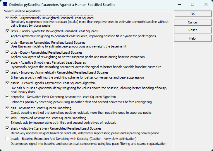
Once you have the best human-engineered baseline you can devise, click the Optimize button. Select the algorithms you wish to train to match your human baseline. Click OK to initiate a set of generic algorithm (differential evolution) optimizations where the parameter(s) of each Whittaker algorithm are optimized to match as closely as possible your human designed baseline. PeakLab launches an embedded python procedure to perform these training optimizations.

Note that you are training these algorithms how to process just this specific type of separation or spectral analyses. Baselines of an entirely different rate of change or data with significantly different S/N, sampling rate, or width of peaks will require separate optimizations.

When the optimizations are complete, you will see a summary similar to the following:

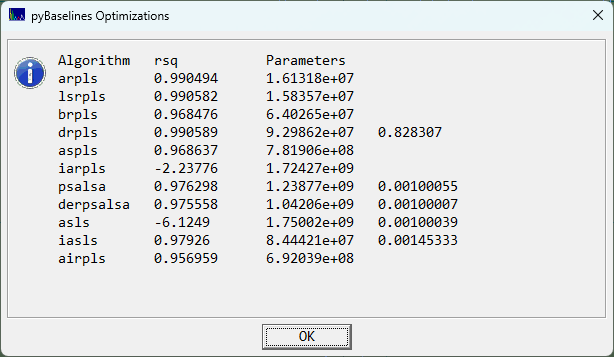
In this example, the arpls, lsrpls, and drpls outperformed the other algorithms in matching the human designed baseline. When you click OK, the parameter(s) for each of the algorithms will be automatically updated in the dialog so that you can view the optimizations.

Choose the Partial option each time it appears so that the human designed baseline is never updated if you wish to keep it displayed. The Whittaker baselines algorithms override your selected points as each determines it own set of peaks and baseline points in the data. Your own specified points or those automatically determined by the selected method are not used, even though they are shown on the plot as a reference.

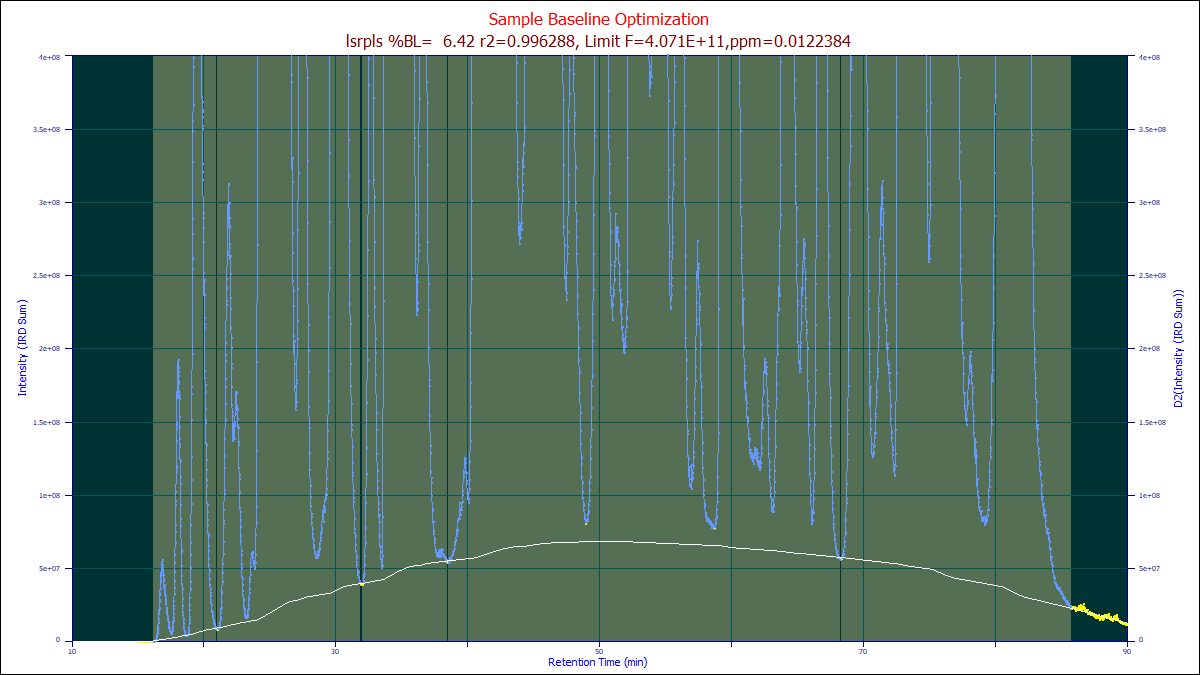
If the arpls algorithm is chosen as the Model after this optimization, the optimized arpls lambda will be used, generating the white baseline above. You can then select all of the different baselines in you wish to see which one best manages your specific baseline.

Optimization of the BEADS Algorithm

All of the Whiitaker algorithms are either order N, or modified for PeakLab to use an order N pentadiagonal solver. Although the Whittaker algorithms are iterativem they converge reasonably swiftly.

The BEADS baseline algorithm, on the other hand, is a computationally expensive DSP procedure that is also offered in the Baseline option. Please be wary of optimizing the BEADS algorithm alongside the Whittaker algorithms unless your data has a reasonably low N. The BEADS is notoriously hard to manually tune, and as such the optimization may be of appreciable value, but it is a very slow iterative algorithm, especially with large data sets, and the GA must optimize five different parameters. It is recommened that you optimize BEADS only if you specifically want to use this algorithm.