PeakLab v2 Documentation Contents R2N Software Home R2N Software Support
Convolutions - Gaussian and Kinetic Decay
In addition to the EMG model, many kinetic decay models have closed form solutions for integer ratios of powers that differ by 1. The following models consist of Gaussian Ä Kinetic Decay for order 0, 1/2, 2/3, 2/4, 4/5, 5/6, 6/7, 7/8, and 9/10. These are significant since catalyzed kinetics have such orders.
As closed form solutions, even the rather onerous orders nearer 1 are computationally fast relative to models which require internally iterative special functions, but there can be precision issues, especially in the orders from 5/6 upward. This is evident in the order 9/10 plots, but can occur with any of the models as the a3 t or time constant approaches 0.
Also note the similarity illustrated at the end of this topic where kinetic and a half-Gaussian probabilisitic decays are compared.
Gaussian Ä Kinetic Decay Order 0
a0 = Area
a1 = Center (mean)
a2 = Width
a3 = Kinetic Time Constant t, order 0
Built in model: KMG[0]
User-defined peaks and view functions: KMG[0](x,a0,a1,a2,a3)
![v5_Convolution_KMG[0].png](v5_Convolution_KMG[0].png)
Gaussian Ä Kinetic Decay Order 1/2
a0 = Area
a1 = Center (mean)
a2 = Width
a3 = Kinetic Time Constant t, order 1/2
Built in model: KMG[1/2]
User-defined peaks and view functions: KMG[1/2](x,a0,a1,a2,a3)
![v5_Convolution_KMG[1_2].png](v5_Convolution_KMG[1_2].png)
Gaussian Ä Kinetic Decay Order 2/3
a0 = Area
a1 = Center (mean)
a2 = Width
a3 = Kinetic Time Constant t, order 2/3
Built in model: KMG[2/3]
User-defined peaks and view functions: KMG[2/3](x,a0,a1,a2,a3)
![v5_Convolution_KMG[2_3].png](v5_Convolution_KMG[2_3].png)
Gaussian Ä Kinetic Decay Order 3/4
a0 = Area
a1 = Center (mean)
a2 = Width
a3 = Kinetic Time Constant t, order 3/4
Built in model: KMG[3/4]
User-defined peaks and view functions: KMG[3/4](x,a0,a1,a2,a3)
![v5_Convolution_KMG[3_4].png](v5_Convolution_KMG[3_4].png)
Gaussian Ä Kinetic Decay Order 4/5
a0 = Area
a1 = Center (mean)
a2 = Width
a3 = Kinetic Time Constant t, order 4/5
Built in model: KMG[4/5]
User-defined peaks and view functions: KMG[4/5](x,a0,a1,a2,a3)
![v5_Convolution_KMG[4_5].png](v5_Convolution_KMG[4_5].png)
Gaussian Ä Kinetic Decay Order 5/6
a0 = Area
a1 = Center (mean)
a2 = Width
a3 = Kinetic Time Constant t, order 5/6
Built in model: KMG[5/6]
User-defined peaks and view functions: KMG[5/6](x,a0,a1,a2,a3)
![v5_Convolution_KMG[5_6].png](v5_Convolution_KMG[5_6].png)
Gaussian Ä Kinetic Decay Order 6/7
a0 = Area
a1 = Center (mean)
a2 = Width
a3 = Kinetic Time Constant t, order 6/7
Built in model: KMG[6/7]
User-defined peaks and view functions: KMG[6/7](x,a0,a1,a2,a3)
![v5_Convolution_KMG[6_7].png](v5_Convolution_KMG[6_7].png)
Gaussian Ä Kinetic Decay Order 7/8
a0 = Area
a1 = Center (mean)
a2 = Width
a3 = Kinetic Time Constant t, order 7/8
Built in model: KMG[7/8]
User-defined peaks and view functions: KMG[7/8](x,a0,a1,a2,a3)
![v5_Convolution_KMG[7_8].png](v5_Convolution_KMG[7_8].png)
Gaussian Ä Kinetic Decay Order 9/10
a0 = Area
a1 = Center (mean)
a2 = Width
a3 = Kinetic Time Constant t, order 9/10
Built in model: KMG[9/10]
User-defined peaks and view functions: KMG[9/10](x,a0,a1,a2,a3)
![v5_Convolution_KMG[9_10].png](v5_Convolution_KMG[9_10].png)
Gaussian Ä Kinetic Decay Order 1 (EMG)
a0 = Area
a1 = Center (as mean of Gaussian peak that is convolved by the a3 exponential)
a2 = Width (SD of the Gaussian peak that is convolved by the a3 exponential)
a3 = The first order kinetic or exponential decay width convolving the Gaussian (can be negative to model fronted peaks)
Built in model: EMG
User-defined peaks and view functions: EMG(x,a0,a1,a2,a3)
![v5_Convolution_KMG[1].png](v5_Convolution_KMG[1].png)
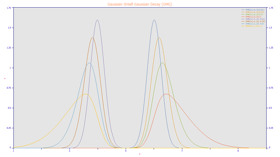
Gaussian Ä Half-Gaussian Decay (GMG)
a0 = Area
a1 = Center (as mean of Gaussian peak that is convolved by the a3 half-Gaussian)
a2 = Width (SD of the Gaussian peak that is convolved by the a3 half-Gaussian)
a3 = The first order probabilisitic half-Gaussian width convolving the Gaussian (can be negative to model fronted peaks)
Built in model: GMG
User-defined peaks and view functions: GMG(x,a0,a1,a2,a3)

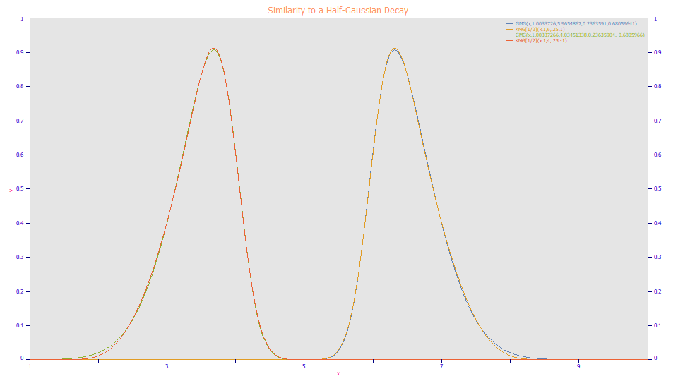
Similarity to a Half-Gaussian Probabilisitic Decay
A half-Gaussian probabilistic decay tends to be quite similar to a kinetic decay with an order in the vicinity of approx 0.55.
The following graph consists of four plots, a fronted GMG and 1/2 order KMG, and a tailed GMG and 1/2 order KMG, the parameters adjusted to produce as close a match as possible. These are very different models which can produce similar shapes.
