Fourier S/N Estimation

PeakLab v1 Documentation Contents AIST Software Home AIST Software Support

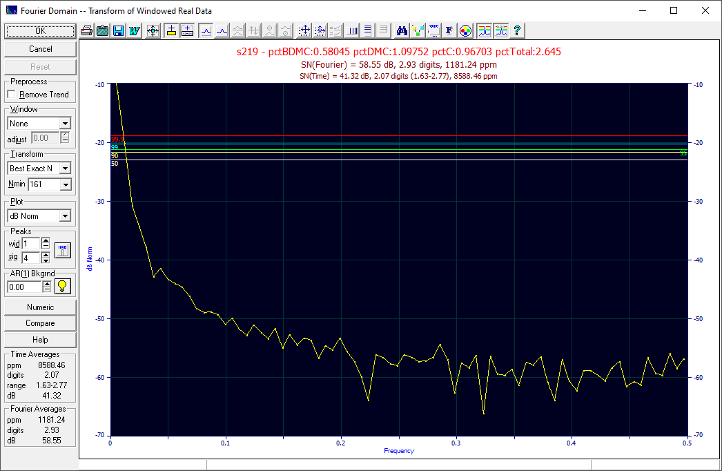
The Fourier S/N Estimation item in the DSP menu opens the Fourier Signal/Noise Analysis procedure:

Although this procedure is designed primarily for S/N estimates, it is a full Fourier analysis procedure with data tapers, different Fourier transform algorithms, variable zero padding, different plots, and critical limits for white and red noise. The data stream should be uniformly sampled (constant sample increment).

Preprocess

The Remove Trend will force the endpoints of the data processed from the Fourier algorithm to begin and end at 0 by subtracting a linear trend.

Window

PeakLab offers a broad selection of data tapering windows to minimize spectral leakage. The adjust field is used to set the spectral width, and thus the dynamic range, of adjustable windows. This field will be disabled for fixed windows.

The spectrum is normalized so that its power equals the power of the input data, regardless of the data window used. In PeakLab, a windowed FFT spectrum will contain the same power as a non-windowed spectrum, and both will match the power in the input data.

Transform

AutoSignal offers the following FFT algorithms:

· FFT Radix 2

· Prime Factor

· Mixed Radix

· Chirp-Z

· Best Exact N

The Best Exact N composite algorithm is the default. If the data size is a power of 2, the FFT Radix 2 algorithm is used. If not and the size is included in the prime-factor set, then the Prime Factor procedure is used. Otherwise, the Mixed Radix algorithm is used if the largest prime <= 509 and the Chirp-Z is used if the largest prime >= 521. This produces the fastest possible exact n FFT.

Nmin

The initial Nmin value will be the data size. To zero pad, enter any value greater than the data size. You may also select from a power of 2 sequence in the drop down box. Note that the actual size of the FFT may be greater than this value if the FFT Radix 2 or Prime Factor algorithm is used.

Increasing the zero padding will increase the number of frequency channels, which for small size data sets can aid in more accurately determining the center frequencies of spectral peaks. This will not change the basic shape of the spectrum, however. If a given peak is defined by only three frequency bins when an exact 64 point FFT is made, a 1024 point FFT will basically fill in this same shape. It is a kind of interpolation since zero padding cannot sharpen the peaks. To achieve this sharpening with an FFT, a longer set at the same sampling rate would be required. For data that are rapidly changing, or when the time series is limited in size, a non-FFT procedure is usually required for good spectral resolution.

When a data tapering window is used, very little spectral leakage arises from the zero-padding.

Plot

The frequency domain information can be plotted in a variety of formats. In the following table, Re is the real component of the FFT at a given frequency, Im is the imaginary component, n is the data set size, dx is the sampling interval, and var is the variance of the data series.

· Real, abs(Re)

· Imaginary, abs(Im)

· Magnitude, sqrt(Re*Re+Im*Im)

· Phase, sine-based, Pi/2+atan(Im/Re)

· Mag/Phase, dual plot, magnitude in Y, phase in Y2

· Amplitude, 2.0*sqrt(Re*Re+Im*Im)/n

· Ampl/Phase, dual plot, amplitude in Y, phase in Y2

· dB, decibels, 10.0*log10(Re*Re+Im*Im)

· dB Norm, decibels, normalized to 0 for frequency channel with maximum power

· PSD SumSq, Power as Sum Squared Amplitude, 2.0*(Re*Re+Im*Im)/n

· PSD MeanSq, Power as Mean Squared Amplitude, 2.0*(Re*Re+Im*Im)/n/n

· PSD TimeInt, Power as Time-Integral Squared Amplitude, 2.0*dx*(Re*Re+Im*Im)/n

· Variance, Power normalized by variance, (Re*Re+Im*Im)/n/var

In an amplitude plot, you see the actual amplitude of sine components. In a normalized decibel plot, the highest peak is at 0dB, a peak at -3dB would have half the power, and a peak at -6dB would have half the amplitude. The PSD TISA (time-integral squared amplitude power) is the actual integral under the curve defined by the square of the raw data.

Peaks

The spectral peaks are identified by a local maxima detection algorithm. Both the amplitude and the frequency locations of the detected peaks are based upon a cubic spline bin interpolation procedure.

The sig item sets the target number of peaks (signal components) to detect. Up to 50 peaks can be detected. Peaks are ranked by interpolated amplitude. Note that this target signal component count may not be realized as fewer peaks than this target may be detected. Note also that the frequency analysis and linear sinusoidal fits reported in the Numeric Summary use the component count and frequencies from this peak identification.

The wid item sets the bin width tolerance for defining a peak. A peak must exist across this number of FFT bins to be counted. The default is a single bin.

The Display Maxima option is used to step through the options for displaying spectral peak labels: frequencies, spectral magnitudes, both frequencies and spectral magnitudes, or none.

AR(1) Background

PeakLab offers peak-type critical limits to determine the statistical significance of the largest peak present in the spectrum. These limits are computed for all windows, including those with adjustable parameters. The default background used for this null hypothesis is white (Gaussian or normally distributed) noise, AR(1)=0.0. A lag-1 autoregressive spectrum can also be specified. An AR(1) coefficient greater than 0.0 can often model red noise (where the noise power decreases with increasing frequency).

The AI Expert option will set the AR(1) value to the lag-1 normalized autocorrelation. This should only be used as a preliminary estimate.

The Show Significance Levels option is in the graph's toolbar. This button is used to toggle the significance levels on and off.

Numeric

The Numeric button opens the Signal Noise Analysis window.

Signal Noise Analysis

Algorithm: Best Exact N

Window: None

Size Size Time Time Time Fourier Fourier Data

Data FFT SNRdb Digits ppm SNRdb Digits ID

161 161 41.3216935 2.06608467 8588.46056 58.5532309 2.92766154 s219

161 161 51.6809324 2.58404662 2605.87379 61.3382564 3.06691282 s220

161 161 41.9321351 2.09660675 8005.58819 65.2179760 3.26089880 s222

161 161 43.7644836 2.18822418 6482.99698 62.7763699 3.13881849 s223

161 161 45.0613650 2.25306825 5583.82435 63.0190151 3.15095076 s224

161 161 45.4617571 2.27308786 5332.27015 64.6110313 3.23055156 s225

161 161 45.5542386 2.27771193 5275.79691 65.2302258 3.26151129 s226

161 161 47.2975383 2.36487691 4316.41394 63.2402817 3.16201409 s227

161 161 47.4876148 2.37438074 4222.98228 61.9017618 3.09508809 s228

161 161 41.6075109 2.08037555 8310.44834 63.7479261 3.18739630 s229

161 161 55.0072352 2.75036176 1776.79875 65.4612237 3.27306119 s230

161 161 52.1091906 2.60545953 2480.50707 64.0886330 3.20443165 s231

Avg 46.5238079 2.32619040 5248.49678 63.2654943 3.16327472 All Data

The PeakLab S/N Analysis consists of both a time domain method which estimates the amount of white noise in the data, and a Fourier analysis procedure which measures the noise floor in the data.

The time domain procedure estimates the level of white (Gaussian random) noise in the data. For each point, a time-domain interpolation is made using adjacent points on each side of that data point, and the difference between that interpolation and the data is treated as the noise predictor at that data value. The average of those absolute differences is input in a predictive model that was built using a large Monte Carlo simulation consisting of different sizes of data and different levels of known white noise.

In this procedure the Time ppm is this computed white noise value based on the average absolute errors in the procedure. In the first sample in the above table you can read the S/N estimate as there existing 8588 ppm or 0.86% white noise in the signal. If that level of noise is converted to significant digits, -log10(0.008588), we have the Time Digits value of 2.066 significant digits. If those digits are converted to dB, we have -20*log10(0.008588), the Time SNRdb of 41.32 dB.

The Fourier procedure measure the noise floor in the Fourier domain. At the highest frequencies, it is assumed the signal consists almost exclusively of noise, a fair assumption for chromatographic and spectroscopic data. In the first sample above, the noise floor occurs at the Fourier SNRdb of 58.55 db in the upper frequencies of this data. This corresponds with 2.927 digits precision, the Fourier Digits in the above table.

The time domain estimate doesn't specify that the noise is white, independent of signal and essentially constant at all frequencies in the Fourier domain. It only means, for this first sample, that 0.86% white noise corresponds with the overall measure of noise in the data. The noise may well be red, higher at lower frequencies where the most of a chromatographic or spectroscopic signal exists and lower at the upper frequencies where no signal exists.

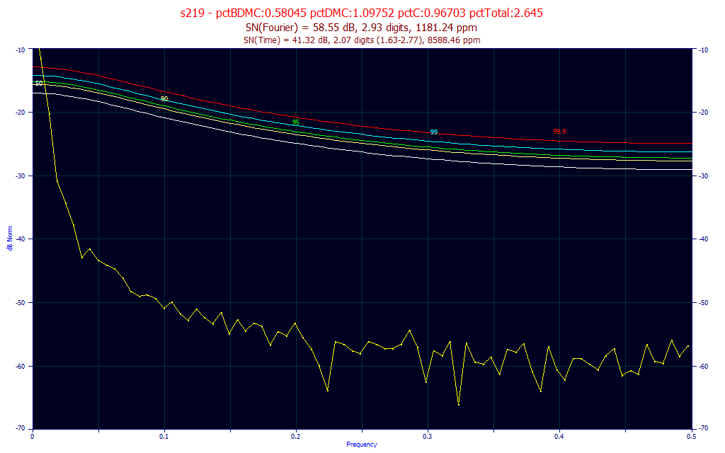
For example, if you look at the critical limit lines for an AR-1 (autoregression order 1) red noise of 0.6, you see a pattern in the critical limits that looks a lot like the pattern in the Fourier spectrum of data from about 0.1 upwards where the noise is apparent. A critical limit is where a spike in the signal appears strictly from random noise. In this example, a 99.9% critical limit, the red line above, means that in 1000 samples of 0.6 AR-1 red noise data sets of this specific size, 1 had its largest Fourier spike at or above this line, and 999 were below.

For this same data, the first image at the beginning of this topic shows the 50, 90, 95, 99, 99.9 critical limit lines for white noise. Note that there is an equal probability at every frequency of having a given level exceeded by random chance. Also note that the uppermost frequencies have lower Fourier thresholds. This should give you some sense for why the estimation of noise can be less than straightforward when this independence between signal and noise is absent.

An overall estimate of white noise in the time domain and the noise floor in the Fourier domain are two different ways to view the noise in spectral data. They should only agree if the white noise (uncorrelated, frequency independent) noise assumption holds.

Compare

The Compare button will open a Fourier plot where multiple data sets can be easily compared with one another.

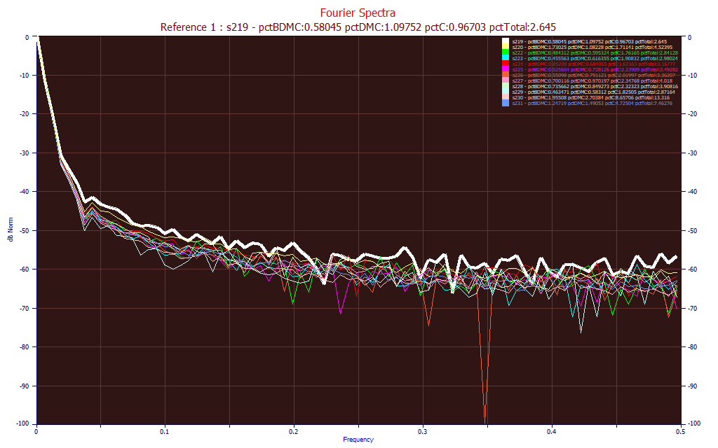
You can select the Use Mouse or Use Legend items to highlight either a curve or legend item to identify the different spectra.

Averages

The dialog will display the averages of multiple data sets as shown in the Numeric option.

Copy An Individual FFT to Clipboard

You can right click any of the Fourier plots and select Copy this FFT to Clipboard to place the a Fourier table on the clipboard.

Save An Individual FFT to Disk

You can right click any of the Fourier plots and select Save this FFT to File to write the Fourier table to disk.

View an Individual FFT

You can right click any of the Fourier plots and select View this FFT in a Numeric Table to open a window containing the Fourier table to disk.

Chnl Frequency Magnitude Amplitude Wavelength Phase dB Norm PSD TISA

0 0.0000000000 30233.900261 187.78820038 0.0000000000 1.5707963268 0.0000000000 5677569.7204

1 0.0062111801 8071.8225520 100.27108760 161.00000000 4.2741443871 -11.47045140 809370.42622

2 0.0124223602 2956.8014353 36.730452612 80.500000000 5.6054297607 -20.19344031 108604.65500

3 0.0186335404 875.37300637 10.874198837 53.666666667 5.7429105065 -30.76602052 9518.9801278

4 0.0248447205 589.17337853 7.3189239569 40.250000000 6.0473059769 -34.20502122 4312.1151549

5 0.0310559006 391.23181422 4.8600225369 32.200000000 0.1400609986 -37.76120025 1901.3954343

6 0.0372670807 219.23615971 2.7234305555 26.833333333 6.0959520813 -42.79163980 597.07445623

7 0.0434782609 255.43358705 3.1730880378 23.000000000 6.1172136056 -41.46432348 810.51325951

8 0.0496894410 207.38381953 2.5761965159 20.125000000 6.2712379888 -43.27438614 534.26147332

9 0.0559006211 189.73983355 2.3570165659 17.888888889 0.0449992849 -44.04671322 447.21993090

10 0.0621118012 178.43017108 2.2165238643 16.100000000 0.0763644023 -44.58051768 395.49473231

...

Sinusoidal Modeling

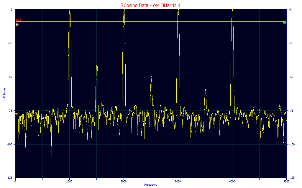
You can right click any of the Fourier plots and select Sinusoidal Modeling of this FFT's Peaks to see a linear multiple sinusoid fit for the peaks in the Fourier spectrum. This is mainly of value for modeling data channels which contain oscillatory components in the Fourier domain. It will not generally be of any value with peak-type data. The following data consists of 7 sinusoids (4 prominent and 3 minor) plus noise. In order to fit this data to seven sinusoids, the sig value must be set to 7:

Fourier Frequency Spectrum

Data: 7Cos1001

X: Frequency

Y: dB Norm

Data Source: C:\PeakLab\Config\CLIPBRD.PRN

Date: Oct 5, 2022

Algorithm: Best Exact N

Window: cs4 BHarris 4

Data Size: 1001

FFT Size: 1001 (7*11*13)

SSA Power: 2000.1851

MSA Power: 1.9981869

TISA Power: 0.20001851

Signal Count: 7

Interpolated Spectral Peaks

Frequency dB Norm

1005.2100405 0.1894634337

1505.2708156 -39.88661372

2005.3347201 0.3216786483

2505.7508840 -49.70352675

3005.3422157 0.1489492234

3505.6778225 -59.32619748

4005.2042014 0.0696866871

Frequency Analysis

Frequency Amplitude Phase Power % Rel %

1005.2100405 0.9872804354 1.2744816397 0.0487848690 24.711366704 97.718227673

1505.2708156 0.0099391605 1.1947412433 4.944285e-06 0.0025044658 0.0099036190

2005.3347201 0.9908999333 1.1542377462 0.0491432280 24.892888975 98.436036397

2505.7508840 0.0032527060 1.0766978791 5.295338e-07 0.0002682287 0.0010606794

3005.3422157 0.9951038027 1.1783240928 0.0495610905 25.104551990 99.273033189

3505.6778225 0.0010776440 1.1488934521 5.812389e-08 2.944193e-05 0.0001164247

4005.2042014 0.9987406811 1.3147948684 0.0499240216 25.288390194 100.00000000

0.1974187410 100.00000000

Sine Component Fit (Suboptimal)

Frequency Amplitude Phase Power % Rel %

1005.2100405 0.9907648074 1.5051935769 0.0490909709 24.994640094 99.719623852

1505.2708156 0.0016254778 1.9196484092 1.321242e-07 6.727096e-05 0.0002683869

2005.3347201 0.9900905630 1.4665705491 0.0490220871 24.959567932 99.579698540

2505.7508840 0.0048723790 4.0752508628 1.187242e-06 0.0006044836 0.0024116721

3005.3422157 0.9905060370 1.4642413224 0.0490606534 24.979203924 99.658039087

3505.6778225 0.0062674530 4.2288279926 1.964364e-06 0.0010001549 0.0039902582

4005.2042014 0.9922347950 1.5071058985 0.0492289973 25.064916140 100.00000000

0.1964059925 100.00000000

r2 DOF r2 Std Err F-stat

0.9895620642 0.9893381657 0.1459578896 4645.4147860

Data Power Model Power Error Power Ratio

0.2000168605 0.1979307490 0.0020877631 94.805174507

Sine Component 1