PeakLab v1 Documentation Contents            AIST Software Home            AIST Software Support

Fourier Estimation of Spectroscopic Resolution

The time domain method of fitting multiple Gaussian peaks to data with an F-statistic optimization for the count of Gaussians is effective, but can be challenging when a great many absorbance peaks are present in the the spectrum. Here we describe a method in the Fourier domain that uses D2 (second derivative data). We will give examples where the smoothing to produce the D2 data stream is varied.

High Resolution Spectra (FTNIR)

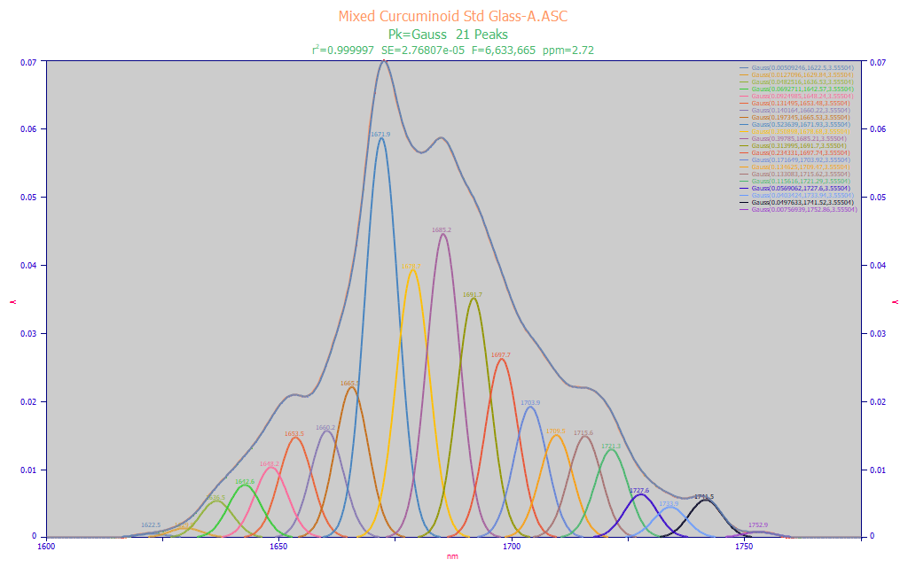
In the Modeling FTNIR Spectra white paper, we performed a shared width multiple Gaussian fit to a three-curcuminoid standard's FTNIR powder reflectance spectra, and estimated the resolution at 3.62 nm, the shared a₂ Gaussian width across the 27 peaks fitted. In this example, to simplify matters somewhat, we use a different run of this same standard and here we baseline correct the data to use only the principal curcuminoid signal between 1620 and 1760 nm.

For practical reasons, we perform the peak fit on wavelength (nm) scale spectra, and the a₂ Gaussian width parameter is shared across all of the fitted peaks. We use that shared a₂ width as an estimate of resolution. A pure spectral fit is often done on a frequency (cm^-1) scale to get the Lorentzian component in Voigt peaks (its width is theoretically proportional to frequency), but such a fit is not possible with this data. The absorbances are many, overlapping, and it is impossible to vary the a₂ Gaussian width of the peaks in the fitting. In the above fit, there are 21 peaks and the a₂ Gaussian width firs to 3.56 nm. The F-statistic is optimized here, 6.63 million, and the error is just 2.72 ppm least-squares error. We believe this to be a good approximation of this FTNIR spectrum's resolution.

FTNIR Spectrum D2 (Second Derivative) Spectrum

The D2 spectra are generated using the DSP menu's Smooth option and selecting the Savitzky-Golay D2 (S-G 2nd deriv) option.

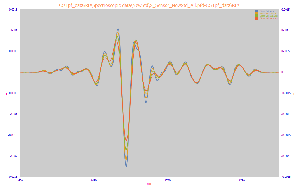
The data was replicated three times using the Replicate this Data Set a Specified Number of Times right click menu option in the main window, and for each of the four identical data sets in the Smooth option, the graph was double clicked and four different smoothing levels were chosen. These are set as a percentage of the data band but the Savitzky-Golay smoothing window sizes are shown in the Smooth option. The above View and Compare Data plot shows the four difference D2 spectra generated for 17, 21, 25, and 29 point two-sided SG windows. These correspond with 8, 10, 12, and 14 point one-sided windows.

FTNIR Fourier Spectral Analysis for Resolution

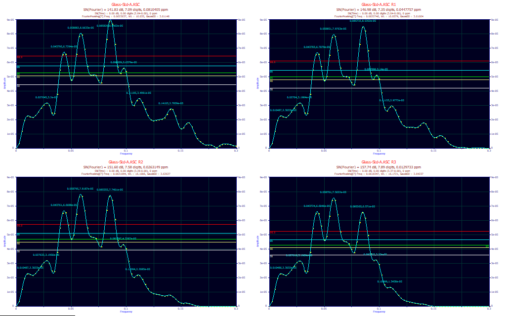
The DSP menu's Fourier S/N Estimation, shown above, is zoomed-in on the X-axis to cover the 0-0.2 frequency band. While there are differences in the Fourier peak areas as a consequence of the D2 smoothing levels, the differences in the peak locations are very small. If we average the first 7 peaks (setting sig to 7), we see in the third title Gaussian SD estimates of 3.611. 3.617, 3.626, 3.642 for the four different smoothing levels. This selects the peaks from the first through where a small plateau first appears at about 0.125 frequency. The third title displays an average frequency, wavelength, and Gaussian SD for the first 7 Fourier peaks. We use an empirically determined Gaussian SD that was found to be the avg wavelength * 0.225. If the peaks are stopped at the 50% critical limit, the estimated Gaussian SD resolution is 4.162-4.186 (sig=6). Please keep in mind that these peaks are estimates of sinusoids. Spectral peak data are neither continuous of waveforms.

Standard Resolution Spectra (UV-VIS)

In the Modeling UV-VIS Spectra white paper, we also performed a shared width multiple Gaussian fit to an average of a large number of turmeric UV-VIS liquid absorbance spectra, and estimated the resolution at 12.64 nm, the shared a₂ Gaussian width across the 9 peaks fitted from 320-480 nm. In this example, we use the same standard as above.

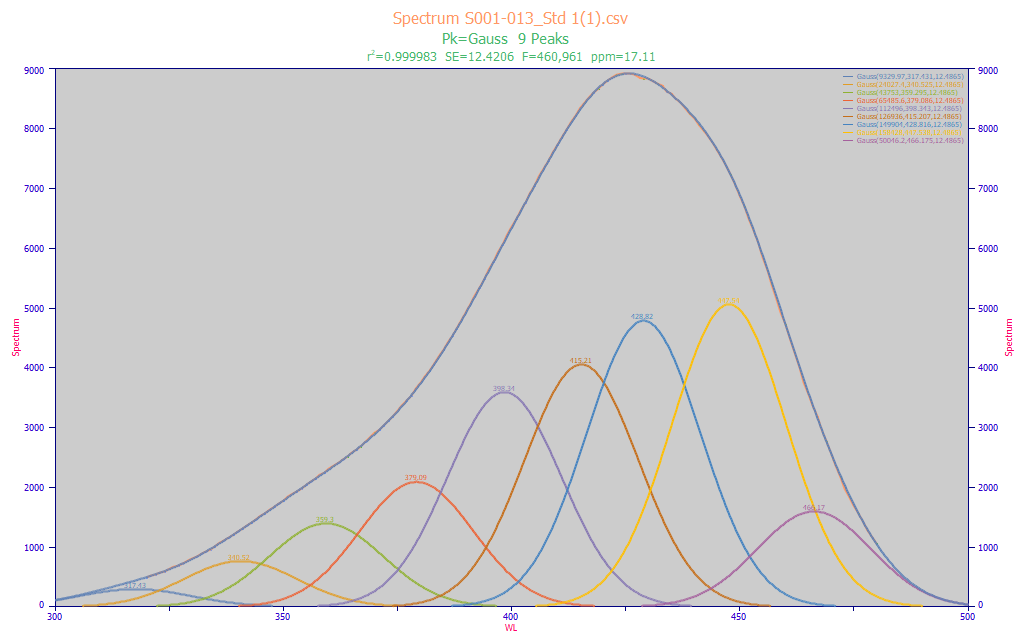
This baseline corrected multiple Gaussian fit to this single spectrum of this standard also optimized to 9 peaks, and an shared Gaussian a2 width of 12.49 nm. As a single spectrum as opposed to an average of many, the fit error is higher, 17 ppm, but the fitted a₁ wavelengths match to within a few nm.

UV-VIS Spectrum D2 (Second Derivative) Spectrum

As in the first example, the D2 spectra are generated using the DSP menu's Smooth option and selecting the Savitzky-Golay D2 (S-G 2nd deriv) option.

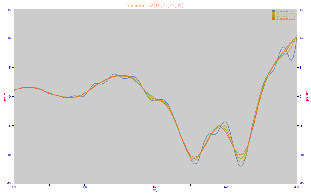
The data was again replicated three times using the Replicate this Data Set a Specified Number of Times right click menu option in the main window, and for each of the four identical data sets in the Smooth option, the graph was double clicked and four different smoothing levels were chosen. The above View and Compare Data plot shows the four difference D2 spectra generated for 19, 23, 27, and 31 point two-sided SG windows. These correspond with 9, 11, 13, and 15 point one-sided windows.

UV-VIS Fourier Spectral Analysis for Resolution

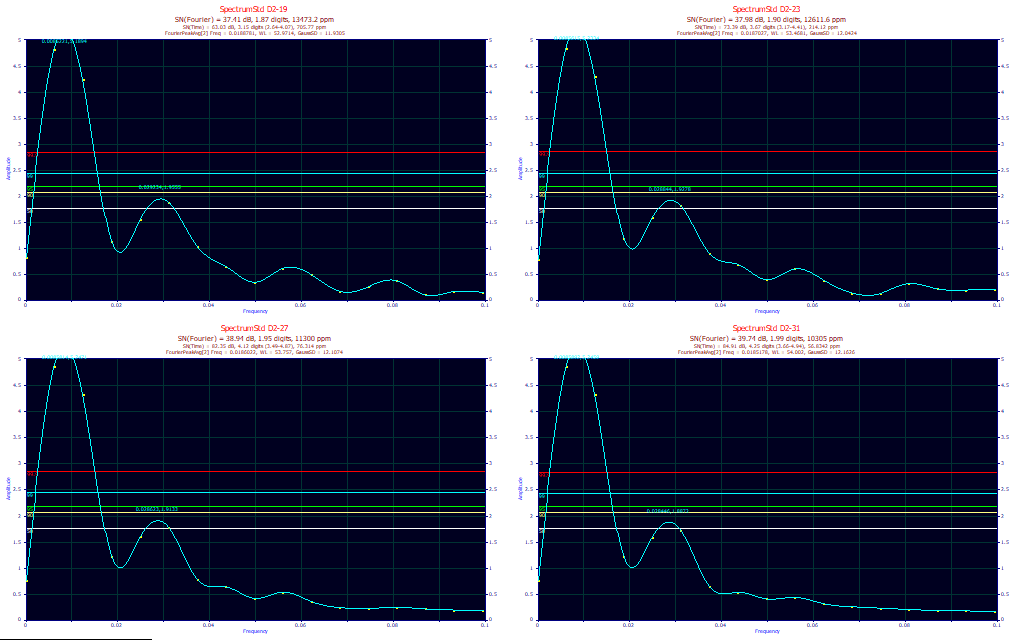
Once more, we use the DSP menu's Fourier S/N Estimation, as shown above. The Fourier spectra are zoomed-in on the X-axis to cover the 0-0.1 frequency band. In this example, we also see a strong consistency in the peak locations. Here, life is simpler, as nearly all of the spectral information rests in just two principal Fourier peaks. If we average the first 2 peaks (setting sig to 2), we see in the third title Gaussian SD estimates of 11.93, 12.04, 12.11, 12.16 nm.

Time Domain Peak Fitting vs. Fourier Estimation of Resolution

The peak fitting approach will likely require more effort as multiple fits will generally be required. You will have to manually remove an added peak that iterates to where it has the same location as an existing peak, and you will have to determine where the F-statistic has its highest value in clean Gaussian count fits. The benefit will be an accurate measure of the resolution as well as estimates of the wavelength values likely to be seen in the spectral modeling.

The Fourier approach is simpler, but there may be an ambiguity with respect to where the Fourier peak count is set. The approach we implement is reasonably insensitive to smoothing levels.

This resolution is important for full permutation spectral modeling. For the FTNIR spectra, we would use an x wavelength spacing of half the 4 nm resolution, every 2 nm. For the UV-VIS spectra, we would use an x wavelength spacing half the 12 nm resolution, sampling every 5 or 6 nm. This understanding of spectral line spreading helps prevent the fitting of noise in all forms of multivariate spectral modeling.