PeakLab v2 Documentation Contents            R2N Software Home            R2N Software Support

Reduce DAD/PDA 3D Matrix

View/Reduce DAD Data Matrix

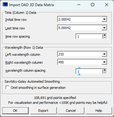
If you wish to visualize portions of the DAD matrix or reduce its size using only a portion of the overall UV-VIS wavelength bands, or reduce the time sampling, you can use the ChromSpec menu's Reduce DAD/PDA 3D Matrix... option. You can use this option to carefully study regions of the chromatographic PDA/DAD spectral-time matrix.

You will want to pay close attention to the size of the grid. PeakLab does not reduce the grid for fast surface rendering. The intention is to model the surface to a high degree of C1 (once continuously differentiable) accuracy. On reason for that is to produce the highest accuracy estimates for the D1 zeroing of components. You will probably find the visualization most palatable if you can keep the size of the grid to no more than 300,000 points. By default, the Agilent UV-VIS ASCII export will have 611 signal values at each time (from 190nm to 800nm at 1 nm intervals). A data set with 10,000 time points will have a 3D spectral matrix with six million signal values. If you used a high sampling rate, you may be able to change the time row spacing. Enter 2 for eery other point, 10 for every tenth point. You should be able to select a start and end time for just the eluted components of interest. In many cases, the wavelength band can be limited to just the UV.

If you wish to have this filtered matrix available for future work, you can use the Export option to save the surface as either a reduced size ASCII matrix, or an ASCII XYZ file (where each entry is a point in the grid).

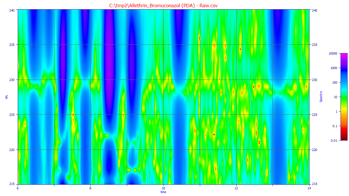
When you click OK, there will be a short delay as the surface is prepared. Unless you check Omit smoothing in surface generation, the matrix will be smoothed in the time dimension using a default Savitzky-Golay denoising filter at each wavelength in the matrix. The surface is then rendered with the Renka C1 triangular surface interpolant. Unless the times and wavelengths have been substantially narrowed, the initial unzoomed plot may contains hundreds of patches (if a patch plot is being rendered). In general, you will need to zoom in the plot to see the time and wavelength regions of interest.

Note that PeakLab automatically creates derivative surfaces when the data matrices are initially imported. For first derivative component zeroing, you can import the first derivative spectra into this procedure to accurately estimate the wavelength(s) where the derivative with respect to wavelength passes through zero. You can use that first derivative spectra and that wavelength in the ChromSpec menu's Import Chromatographic Data Sets option to generate the chromatograms where all components absorbing at one or more central wavelengths are erased from the data.

Options of interest may be:

The Modify Contour Properties button in the graph toolbar opens the option to turn the patch plot option on and off and to set the resolution of the contour plot.

The Overlay Data on Surface or Contour button in the graph toolbar displays and hides the normalized traces of the chromatography.

The 2D View options can be used to set a stronger line width and anti-alias to better see the traces.

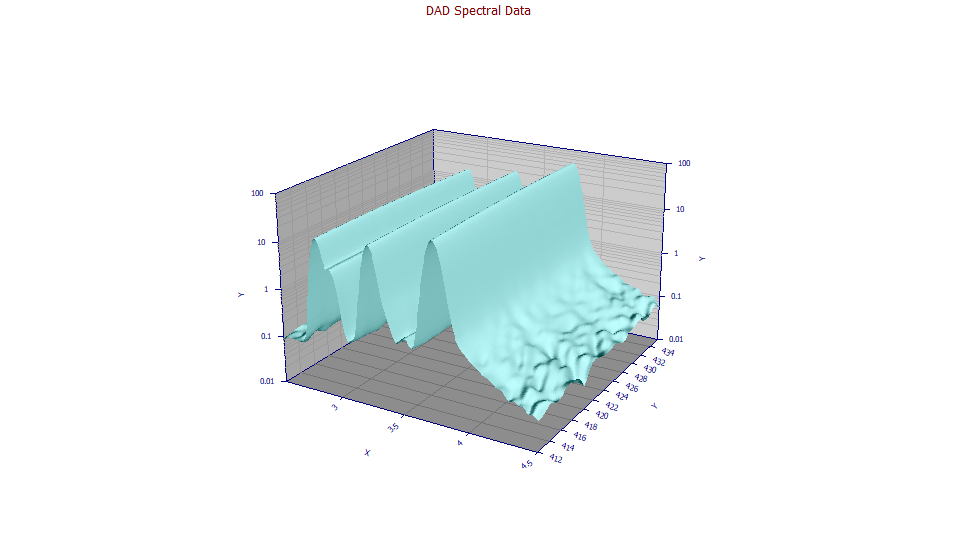
You can use the 3D gradient and shaded options with the 3D animation to better visualize the surfaces.

You can use the Render 3D Surfaces with Plateau at Upper Z Bound to close the surface at the rendering bound

The Logarithmic Z Axis will possibly highlight trace components in the baseline at certain wavelengths and times:

The Force | Zmin = 0 will set the lower limit of the plot at a fixed 0.0, ignoring negative values. This is also useful for seeing peaks in the baseline.

The Force | Zrange = -1,1 will set the lower limit of the plot at a fixed -1 and the upper limit of the plot at +1. This will typically amplify baseline detail.

Extrema

The initial values in the Extrema section will represent the incoming data matrix values. When the plot is zoomed, and the Update button is clicked, the minima and maxima will be updated for the for the zoomed surface with the narrower bounds and the higher resolution. The extrema are based on the values taken from a 250,000 point grid based upon the zoomed x and y ranges. The actual values of these extrema will depend (1) on the optimal Savitzky-Golay filter applied to the incoming DAD data (if used), (2) on the 250,000 point (500 x 500) evaluated Renka C1 3D interpolated surface (this resolution is independent of the grid used for the rendering of the contour or 3D surface plot), and (3) on the level of zoom which determines the x and y bounds of that 250,000 point grid.

If you place the cursor near a minimum or maximum, a local measurement will be made to determine the precise time and WL locations for the minimum and maximum in the region of the mouse cursor, and those will be displayed in the hint popup that follows the mouse cursor.

Partial Derivative Surfaces

The Renka 3D rendering algorithm offers a C1 partial derivative surface with respect to either time (dZ/dX) or wavelength (dZ/dY). These are useful for visualization, and can often have a good accuracy in estimating the wavelengths where the first derivative with respect to wavelength are zero if you are looking at non-derivative data.

Export

This option will export the data matrix used for the extrema computations. It will always consist of 500 equally spaced wavelengths, and 500 equally spaced time values, within the zoomed in region that is plotted. The initial values in the Extrema section will represent the incoming data matrix values. You can save a matrix or a table of XYZ values. Although you can use this option to export a first partial with respect to wavelength surface for derivative fitting, we recommend the next procedure for best accuracy in estimating coeluting peak areas.

Create First Derivative DAD Matrix

Please see the Fitting Coeluting Peaks tutorial for a using identified zero first derivative wavelength values for estimating the areas of coeluting peaks with slightly different UV-VIS spectra.