PeakLab v1 Documentation Contents            AIST Software Home            AIST Software Support

Modeling Spectra - Part I - UV-VIS Data

Authors: Amruta Behera¹ (amruta.behera@plaksha.edu.in), Hasika Suresh² (hasika.suresh@tufts.edu), Rudra Pratap³ (rudra.pratap@plaksha.edu.in), Ron Brown⁴ (ron@aistsoftware.com)
Publish Date: January 2023.

¹Amruta Behera is a founding professor at the new Plaksha University in Mohali, the planned city in the Punjab near Chandigarh, India. Amruta managed the project where the data shown in this white paper was generated as part of his several years of post-doctoral research at the Indian Institute of Science (IISc) in Bangalore, India. In this project, handheld spectrometers were designed, built, and tested for in-field analysis of spices and other cultivated botanicals.

²Hasika Suresh is a doctoral student in the department of Chemical and Biological Engineering at Tufts University, Boston. While she was at the Centre for Nanoscience and Engineering (CeNSE) at IISc India, she developed the HPLC methodology for curcuminoid and turmeric samples and worked to procure a vast library of turmeric roots and powders. Hasika generated all of the chromatographic data illustrated in this white paper.

³Rudra Pratap is the founding vice chancellor (president) of Plaksha University. Prior to this position, Rudra served as the Deputy Director of Indian Institute of Science, Bangalore, India where he founded of the IISc Centre for Nano Science and Engineering (CeNSE) and where, for a time, he served as chairman of the board of a major scientific and statistical software company. In an effort to create tools for Indian farmers growing spice crops to better quantify the value of their harvests, Rudra created and guided the R&D project that resulted in all of the chromatographic and spectroscopic data that appears in this series of modeling white papers. The samples analyzed in these white papers were collected across several years and now represent what we believe to be the most comprehensive and diverse library of commercially grown turmeric in the world.

⁴Ron Brown is the founder of AIST Software, in Oregon, USA, and the author of the PeakLab software, as yet unreleased, which was used to analyze much of this data that appears in these white papers. Ron developed the original PeakFit software and also authored the TableCurve software products for curve and surface fitting as well as AutoSignal for signal analysis.

A Novel Approach for Generating UV-VIS Models of Turmeric and Other Botanicals

In this first white paper, we describe a method to explore the viability of UV-VIS models using spectra reconstructed from an HPLC instrument's DAD (diode array detector). We will create models for the total curcuminoids and for the three principal curcuminoid components in turmeric powders.

Using the DAD 3D Time-Wavelength Spectra from the Chromatography

A modern HPLC instrument allows the full 3D time-wavelength spectra from the DAD to be saved as an ASCII file for further processing. If the laboratory reference variables for the modeling are derived from chromatographic separations, we found it to be a simple matter to do this form of model exploration since the chromatography furnishes both the species quantities (Y-values) and the UV-VIS spectra (the X-predictors).

The advantages include the simplicity of one prep and one instrumental analysis and a complete correspondence between the chromatography and the UV-VIS spectroscopy. The prep for the chromatography will necessarily address all issues of solubility with respect to an extraction procedure of solid materials since the the spectroscopy solvent is the mobile phase of the chromatography.

The main disadvantage of this approach as an exploratory modeling methodology is the need to isocratically clear everything off the chromatographic column that exists within the UV-VIS wavelengths that will be used for the modeling. In order for the reconstructed UV-VIS spectra to be valid, everything in the wavelength band for the modeling must elute between the dead time of the column and the point where the chromatographic run ends. Also, since the spectral absorbances will vary in both magnitude and frequency with the state of the solvents, a gradient separation cannot be used, nor a separation with a flush step of different concentration of the solvents as the last part of an otherwise isocratic run if any of the content in this last step contains spectral signal in the wavelengths of concern. We have also confirmed that the signal/noise is lower in this form of UV-VIS reconstruction than would be seen from a dedicated UV-VIS laboratory spectrometer. Also, for long chromatographic separations, there may be a drift in the spectroscopy baselines at the different wavelengths which may require a baseline correction at each wavelength before the reconstructions are done.

HPLC method

An Agilent 1260 Infinity II series chromatograph was used with an Infinity Lab Poroshell 120 EC C-18 UHPLC column, 4.6*50 mm, 2.7 micron, to produce the separation of the curcuminoids. The separations were isocratic using a mobile phase of 0.2% orthophosphoric acid : acetonitrile at a 55:45 (v/v) ratio. The separations were carried out at a flow rate of 0.8ml/min, a temperature of 40C, and an injection volume of 20 µl. Concentrations and run times varied depending on the materials and the objectives of the separations. For most runs, the three principal curcuminoids would elute quite swiftly, between 2.5-4.5 minutes.

A Chemstation contributed macro, export3d.mac, was used to export the Agilent 3D DAD data to an ASCII CSV file.

Chromatography and Reconstructed UV-VIS Spectra

In the data we used for this modeling, we reconstructed UV-VIS spectra from the DAD for the time ranging from 45 seconds, just past the dead time of the column, to 6 minutes, the time in the chromatographic separation where no further 300 - 500 nm information (the modeling band) would be seen in the elutions. In order to be certain the reconstructed spectra represented a fair approximation of a laboratory UV-VIS spectrometer, we ran 1-hour separations on a number of representative turmeric samples and confirmed that the last trace of 300+ nm UV-VIS signal ended at approximately 5 minutes in the elution. All later eluting peaks were higher MW oils and turmerones that absorbed well below 300 nm in the UV (the turmerones, present in turmeric at approximately the same levels as the curcuminoids, have their peak absorbance at about 240 nm).

We thus reconstructed the UV-VIS spectra by summing the DAD signal values from 45 seconds to 6 minutes in the chromatographic 3D data matrix, irrespective of the actual length of the chromatographic run.

Understanding the Chromatography

To fully understand the dependent variable(s), the Y values containing the chromatographic estimates of total and component curcuminoids, we ran the chromatography for three analytic standards representing the principal curcuminoids in commercially grown turmeric.

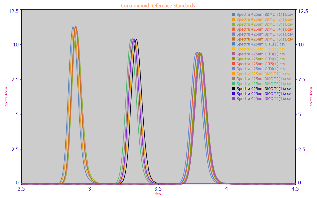
Fig. 1 Area-normalized chromatographic peaks of pure reagent grade BDMC, DMC, and curcumin - six replicates each, overlaid on a single plot for comparison

The first component shown in the Fig. 1 area-normalized comparison plot is BDMC, bis-demethoxycurcumin, usually the smallest component of the three principal curcuminoids. The second peak is DMC, demthoxycurcumin, and the third is curcumin, usually the largest of the three components. In turmeric, a natural botanical, there a number of curcuminoids besides these three. We observed all to elute either in the range of these three (one approximately coeluting with the BDMC), or earlier in time as a consequence of having a greater hydrophilicity.

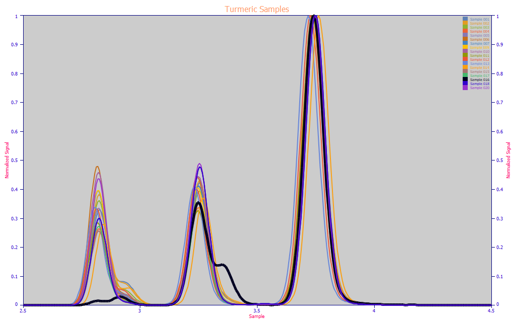
Fig. 2 Area-normalized chromatograms of eighteen different turmeric samples

The turmeric chromatography in Fig 2. illustrates a companion peak in the right shoulder of the BDMC peak which is present to some degree in every sample. Also shown above, in the highlighted black curve, is an aromatic turmeric which is a different species of turmeric from the one used as a spice and medicine; it contains a DMC coeluting peak. In the chromatographic computation of total curcuminoids, these companion peaks were added to the total curcuminoids if they were not already integrated together with the BDMC or DMC peaks.

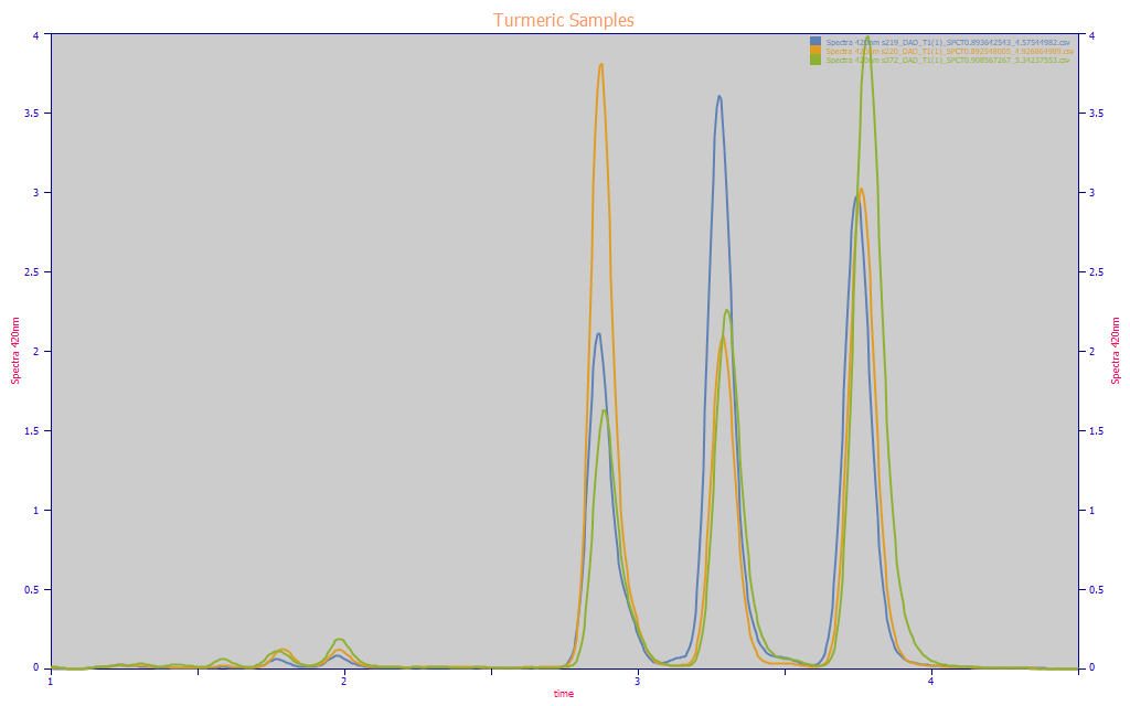
Fig. 3 Area-normalized chromatograms of three turmeric samples illustrating extremes of component fractions and traces of hyrdophilic curcuminoids at early elution times

The Fig. 3 plot illustrates very small concentrations of much more hydrophilic curcuminoids at lower (1.6-2.0) elution time values. These also absorb in this blue 410-440 nm curcuminoid region, and could be, in rare cases, as high as 2-3% of the total curcuminoids. We made a conscious choice to neglect these trace components since they were rarely included in the chromatography instrument's default integration, appreciating that this would represent a small inherent error between the chromatography and spectroscopy. The same is true for peaks that were sometimes observed between the primary peaks, as in the blue curve.

Although the curcumin component was typically the largest of the three components, the spectral modeling must ideally bracket all bounds on naturally occurring turmeric. In the above area normalized plot, you see an instance where the DMC is the largest component (blue) and where the BDMC is largest (amber).

Any predictive model that fails to bracket the extremes that occur in nature will likely perform poorly near such bounds. We will note that many published papers on spectral modeling of turmeric little addressed such bracketing. We had collected over 200 discrete turmeric samples in our library before adding the amber and blue extremes shown in the above plot.

Understanding the Spectroscopy

To fully understand the spectroscopy or the X-predictors in the modeling, we need a clear picture of where each of the principal curcuminoids absorb in the UV-VIS, and ideally we would also like to know the spectra for the secondary curcuminoids, even though they will be present at much lower levels.

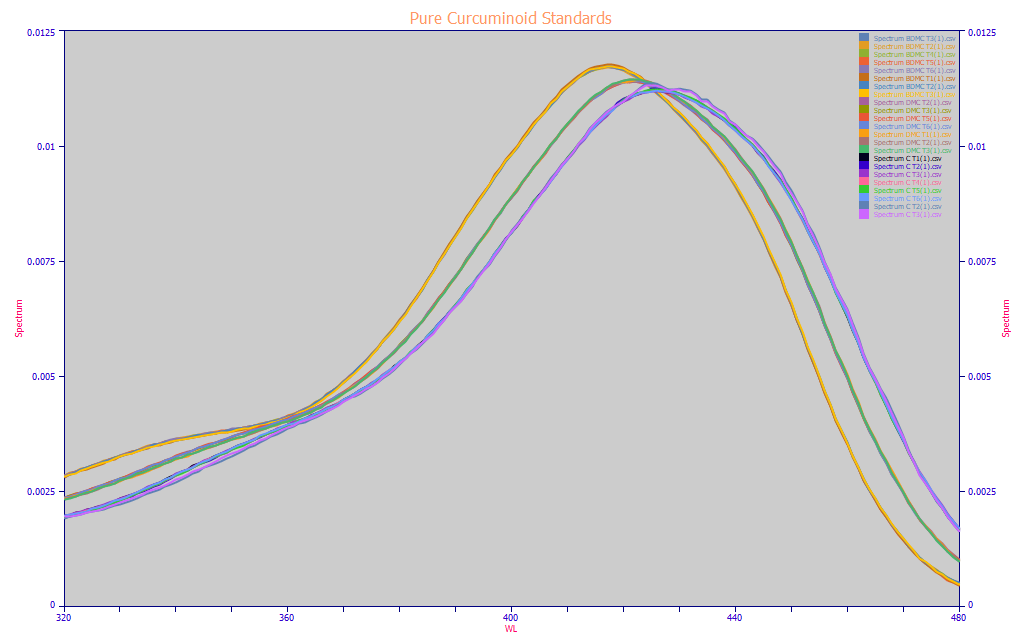
Fig 4. UV-VIS Reconstructions of the chromatography of the BDMC, DMC, and curcumin analytic-grade reagents

Fig 4. contains the full-elution reconstructed UV-VIS spectra from these three reagent grade analytic standards from 320-480 nm. The three principal curcuminoids all have approximately the same spectral absorbances. The BDMC peaks at 417 nm, the DMC at 423 nm, and the curcumin at 426 nm. In this white paper, in addition to fitting total curcuminoids, we will also fit the BDMC, DMC, and curcumin components. If you look closely, you will see that the components are most differentiated from one another at the 320-340 nm and 390-405 nm UV wavelengths and the higher 450-470 nm blue wavelengths, and least differentiated in this area normalized plot at the 425 nm typically used as the central region of absorbance for curcuminoids.

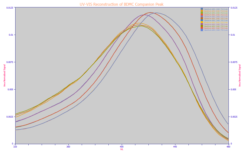
Fig 5. UV-VIS reconstructions of the chromatography from a single turmeric sample, three replicates, the BDMC, DMC, curcumin, and BDMC companion peak

For this type of spectral characterization, needed only to understand the modeling, we will note that it is not necessary to purchase costly analytic-grade reagents to see the individual UV-VIS spectra of each component separated by the chromatography. The spectra at the different times in the chromatography will accurately reveal the UV-VIS spectra of the different components. The Fig. 5 plot, for a single turmeric sample, contains time-window UV-VIS reconstructions from the DAD where each is specific to the time period of elution for a given component. You could possibly see this as a software form of autosampler. The three principal curcuminoids were isolated and reconstructed for their specific time of appearance within the elution. The unidentified BDMC companion peak shown in Fig. 2 was also isolated. The plot reflects three chromatographic replicates for this specific turmeric. The primary curcuminoid components almost perfectly overlap. The very low signal (and only partially resolved) BDMC companion peak, varies somewhat across the replicates, but consistently absorbs at about 412 nm and has an appreciably higher 320-360 nm UV absorbance.

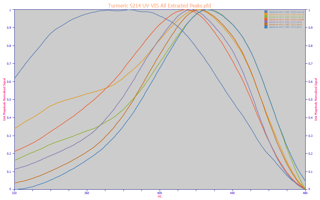
Fig 6. UV-VIS reconstructions of the chromatography from a single turmeric sample, all chromatographic components having an absorbance in the 320-480 nm modeling band

A reconstructed spectra of the components as they eluted in the chromatographic separation gives a clear picture of what the modeling algorithm must include for a total curcuminoid model. In Fig. 6, the three principal curcuminoids, those with the lowest 320-360 nm UV magnitudes, are shown with four other blue-absorbing components isolated in the chromatography. With just one exception, all of these components have a central absorbance between 412 nm and 426 nm and are assumed to be curcuminoids. The spectral feature that is the exception is the very tiny peak that sometimes appears between the DMC and curcumin peaks (for example, the blue curve in Fig. 3). Spectrally, this component is a broad feature with a 370-385 nm UV central absorbance, but it also has a significant yellow color as well, absorbing well into the blue. Although we suspect this trace spectral content is probably not a curcuminoid, it is a small complication a total curcuminoids model will have to sort in certain turmeric spectra. We also note that this represents a small error in both the Y values (chromatography) and the X values (spectroscopy).

Gaussian Peak Fitting - What to Expect in Spectral Modeling

We have found it very useful to use nonlinear Gaussian peak fitting to get a clear picture of the spectral information linear models are capable of recognizing.

Fitted Parameters

r² Coef Det        DF Adj r²          Fit Std Err        F-value            ppm uVar

0.99999444         0.99999369         0.32240197         1,419,179          5.55873539

 Peak        Type               a0                a1                a2  

    1        Gauss        803.114100        314.353709        12.6377393  

    2        Gauss        1653.98689        336.842546        12.6377393  

    3        Gauss        2604.38283        356.378765        12.6377393  

    4        Gauss        3656.61369        377.124828        12.6377393  

    5        Gauss        6305.09912        397.800064        12.6377393  

    6        Gauss        8385.07728        417.587723        12.6377393  

    7        Gauss        5797.13496        432.938890        12.6377393  

    8        Gauss        6519.59429        448.435857        12.6377393  

    9        Gauss        1829.94411        466.607107        12.6377393 

 Measured Values

 Peak        Type          Amplitude          Center             FWHM             Asym50           FW Base            Asym10    

    2        Gauss        52.2122899        336.842547        29.7596018        1.00000000        59.5700398        1.00000000  

    3        Gauss        82.2139466        356.378765        29.7596018        0.99999997        59.5700398        0.99999998  

    4        Gauss        115.430282        377.124830        29.7596018        0.99999980        59.5700398        0.99999989  

    5        Gauss        199.036440        397.800064        29.7596018        1.00000000        59.5700398        1.00000000  

    6        Gauss        264.696229        417.587724        29.7596018        0.99999999        59.5700398        0.99999999  

    7        Gauss        183.001258        432.938893        29.7596018        0.99999972        59.5700398        0.99999985  

    8        Gauss        205.807517        448.435857        29.7596018        1.00000007        59.5700398        1.00000004  

    9        Gauss        57.7668239        466.607108        29.7596018        1.00000000        59.5700398        1.00000000  

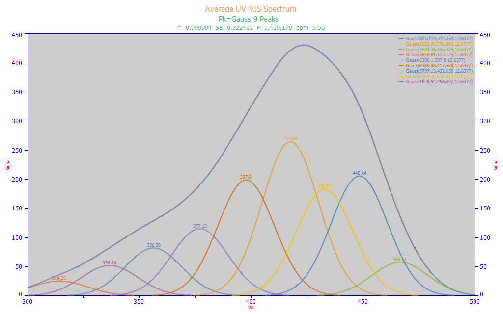
Fig 7a. PeakLab fit of Gaussians to the average spectrum from 156 turmeric samples

We performed a simple multiple Gaussian peak fit where we fit wavelength (nm) instead of frequency (cm^-1) and where, by necessity, a single fitted width is shared across all peaks. We used a spectrum that consists of the average of all 156 turmeric samples we use in this example of UV-VIS modeling. In optimizing the fitting for the count of peaks in the 320-480 nm modeling band, we used the peak fit shown in Fig. 7a that produced the highest F-statistic. In this instance, we have 9 Gaussians with an a₂ SD width of 12.64 nm, corresponding with a FWHM (full width at half-maximum) of 29.76 nm, and a base width (10% of maximum) of 59.57 nm.

We perform this type of fitting to ascertain two important pieces of information. First, the width of the Gaussian peaks helps us to understand the spacing for the predictors used in the full permutation predictive modeling. In this case, there is no need to fit a spectral model using the full permutation algorithm where predictors are spaced 1 nm or 2 nm apart. A spacing of 5 nm is realistic, given this estimated peak width. If desired, the linear modeling can readily generate parameters further refined to the smallest wavelength spacing to see if the additional wavelength resolution offers any significant benefit. In our experience, a simple rule of thumb is to use an x-spacing in the predictors that is approximately half the Gaussian SD of the spectral peaks. In this case, it would be approximately 6 nm. Although the retained full permutation direct spectral fits rarely consist of fitting noise, such can still occur if the spacing is too narrow, and further, a high count of closely spaced predictors will produce seriously lengthy full permutation modeling times for no useful purpose.

Second, the center values of the fitted Gaussians represent wavelengths we might reasonably expect to see in the modeling. The peaks shown in this fit are only approximations, apply only to this averaged spectrum of all of the turmeric samples, and may not correspond exactly with the pure components which produce the overall spectral absorbances. This does, however, approximate what the linear modeling algorithms will be able to see and process. In this instance, we have three main UV wavelengths 336, 356, and 377 nm. There is one transition wavelength at 398 nm. There are three main visible wavelengths at 418, 432, and 448 nm. As you will note, the fit is a strong one, 5.56 ppm statistical (r² or normalized least squares) error. We would thus expect an effective predictive model to incorporate one or many WLs close to these values. The 418 nm peak has the largest amplitude and corresponds closely with the curcuminoid central absorbance. The 448 nm peak has the next highest amplitude.

We stress that this type of peak fitting is not used in the predictive modeling. None of the information from these fits is used as predictors in the modeling. This type of analysis merely gives us a sense for the wavelengths we might expect to see in linear predictive models, as well as a reasonable wavelength spacing for fast full-permutation fitting.

Voigt Peak Fitting - A Refinement in Expectation

The Voigt model is a convolution of a natural spectral line shape, the Lorentzian, and an IRF (instrument response function) broadened Gaussian. It is instructive before we proceed with the direct spectral fits, to validate the wavelengths and width using the Voigt model. We will use a Voigt model that directly fits the Gaussian and Lorentzian widths. Both will necessarily be shared across all peaks in the broad spectral feature.

Fitted Parameters

r² Coef Det        DF Adj r²          Fit Std Err        F-value            ppm uVar

0.99999546         0.99999482         0.29224716         1,636,257          4.53536262

 Peak        Type                      a0                a1                a2                a3    

    1        VoigtGL[amp]        26.2654294        319.880673        10.6293060        2.83945983  

    2        VoigtGL[amp]        52.5384132        340.266173        10.6293060        2.83945983  

    3        VoigtGL[amp]        75.6456418        358.457037        10.6293060        2.83945983  

    4        VoigtGL[amp]        105.060579        377.670439        10.6293060        2.83945983  

    5        VoigtGL[amp]        175.972544        396.595461        10.6293060        2.83945983  

    6        VoigtGL[amp]        230.649597        414.337809        10.6293060        2.83945983  

    7        VoigtGL[amp]        224.971655        429.492858        10.6293060        2.83945983  

    8        VoigtGL[amp]        213.308131        446.473722        10.6293060        2.83945983  

    9        VoigtGL[amp]        73.4504597        462.820871        10.6293060        2.83945983  

Measured Values

 Peak        Type                 Amplitude          Center             FWHM             Asym50           FW Base            Asym10    

    1        VoigtGL[amp]        26.2640873        320.000005        28.1998166        0.98321536        60.1417208        0.99130622  

    2        VoigtGL[amp]        52.5384132        340.266172        28.1987425        1.00000001        60.1411801        1.00000000  

    3        VoigtGL[amp]        75.6456418        358.457037        28.1987425        1.00000000        60.1411801        1.00000000  

    4        VoigtGL[amp]        105.060579        377.670439        28.1987425        1.00000000        60.1411801        1.00000000  

    5        VoigtGL[amp]        175.972544        396.595461        28.1987425        0.99999997        60.1411801        0.99999998  

    6        VoigtGL[amp]        230.649597        414.337809        28.1987425        1.00000000        60.1411801        1.00000000  

    7        VoigtGL[amp]        224.971655        429.492858        28.1987425        1.00000000        60.1411801        1.00000000  

    8        VoigtGL[amp]        213.308131        446.473722        28.1987425        1.00000001        60.1411801        1.00000000  

    9        VoigtGL[amp]        73.4504597        462.820872        28.1987425        0.99999995        60.1411801        0.99999998  

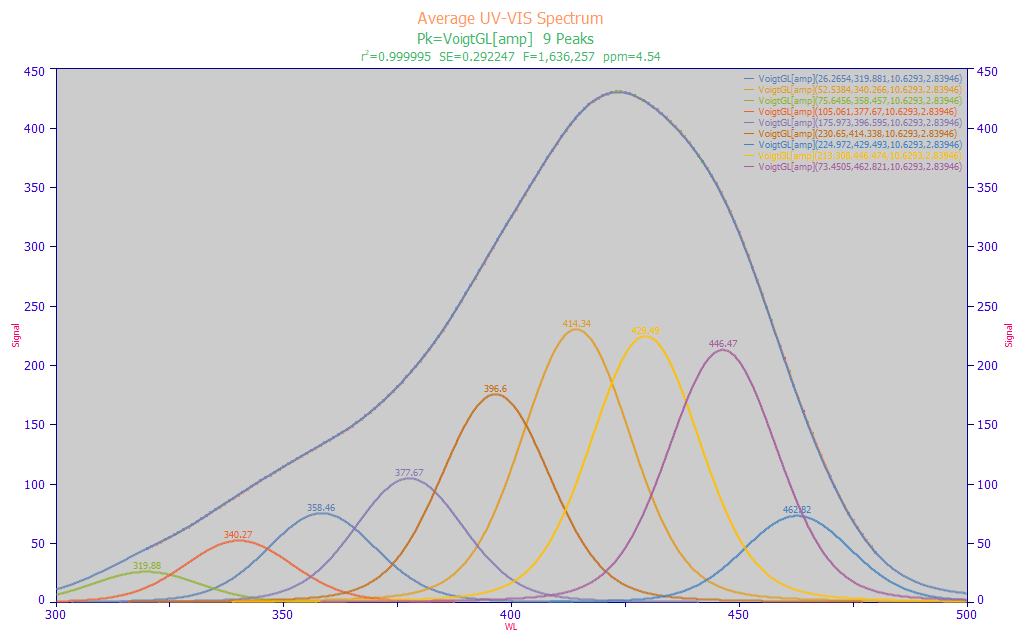
Fig 7b. PeakLab fit of Voigt peaks to the average spectrum from 156 turmeric samples

A close-to-optimal Voigt fit, shown in Fig. 7b, does produce a better F-statistic (assumed to better describe the data), and there is a slightly better 4.53 ppm statistical error. Here we want to point out the shared a2 Gaussian width of 10.6 nm, and the shared a3 Lorentzian width of 2.84 nm. When fitting discrete spectral peaks, such is generally done on a frequency (cm-1) scale since the natural line broadening (the Lorentzian width) will increase proportional with energy. The Gaussian component, when it is only an instrumental broadening, may be independent of frequency. We note that the reason such wavelength (nm scale) fits work to produce such superb fits is that the Gaussian width is much larger than the Lorentzian width.

Because of the additional fitting accuracy with the Voigt, it is useful to compare the estimated wavelengths in the two 9-peak fits:

As you will note, the differences are small and in general, Gaussians should suffice to give a clear picture of the wavelengths likely to be seen in the direct spectral modeling.

Direct Spectral Fit of Total Curcuminoids

We will now begin the predictive modeling.

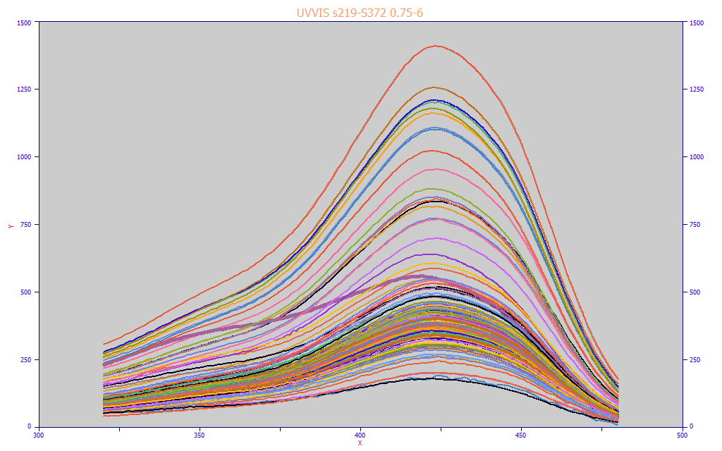
Fig 8. The modeling data matrix plotted as raw individual turmeric spectra with no normalization

Our data matrix for this modeling, shown in the Fig. 8 graph, consists of 156 spectra, each an average of three UV-VIS reconstructed chromatography replicates. As you will note, most track the same general spectral shape, but there are deviations (we highlight the lavender colored spectra above which has a high UV absorbance but a lower visible absorbance). This is a complete map of the predictors, and what the modeling algorithm must sort or unscramble. In our modeling, the Y-values consist of dry-solids adjusted values of the total curcuminoids from the chromatography; moisture differences in the turmeric powders have thus been eliminated in the modeling.

In our experience, we prefer to carry out the modeling with no more than about 100 candidate spectral predictors. In a 5 nm spacing of predictors, for example, this will allow a 500 nm coverage and it will be possible to fit every permutation through eight predictors in a reasonably brief time. In our fit of this UV-VIS data matrix shown above, we fit 320-480 nm models with a 5 nm spacing. We did not need to use filters on the higher predictor count models to hasten the full permutation fitting. We fit every permutation through 8 predictors, approximately 20 million models in all. This required about 10 seconds on a basic 4-core i7 machine (if you have an 6, 8, 12, or 16 core processor, the fitting time will be proportionately faster).

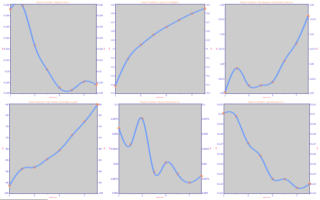
Fig 9. The performance metrics for the full permutation total curcuminoids UV-VIS modeling

Just as with PLS (partial least squares) fits, where a factor or latent variable count must be optimized and is not always straightforward, a direct spectral fit's optimal number of predictors may equally be far from clear. In Fig. 9, we look at the performance stats for an average of the best three retained fits at each predictor count from 1 to 8.

We used the leave one out prediction criterion (it is probably the only prediction algorithm likely to be consistent across different statistical and modeling software). In the leave one out estimate of prediction, a separate fit is made for each spectral set in the data where that specific spectrum is left out of the fitting, and then subsequently tested for prediction after the model using all other spectra is computed. With 156 spectra in our example, there are 156 separate fits, each with one of the spectra removed from the modeling and which estimates a specific error for that specific spectrum. The final prediction performance is based on the errors from the 156 different predictions from the 156 separate models, none of which will exactly match the fitted model being evaluated where no spectrum is left out.

The SE (standard error) in the first panel is lowest (lower is better) at 6 predictors. This SE plot ranges from .156 to .148, about a 5% improvement with the higher parameter count models.

The next panel consists of the log₁₀ (1/F-statistic). This parameterization was done so that this metric will have the same direction as the error and information criteria (where lower is better). The F-statistic shows a clear preference for a 1 predictor model. The F-statistic is a very conservative metric with respect to the count of parameters within a model, one with a very long history amongst statisticians.

The third panel contains the BIC (Bayesian or Schwarz Information Criterion) and it shows an optimum at 3 predictors. The fourth panel contains the MDL (Minimum Description Length). The MDL, although not as widely used, is at attractive criterion since it implements the F-statistic in its theory, and it indicates a single predictor to be optimal.

The last two panels show the median and average absolute prediction errors. These are robust error estimates (as compared to the standard error which uses squared errors), and they both indicate the smallest errors of prediction to occur at 7 predictors. The range of median error covers about a 10% improvement, the range of average error about a 6% improvement.

Our experience with predictive modeling suggests that it is usually best to use the smallest effective predictor count possible in any predictive model. We also favor the MDL which suggests a single predictor suffices. We thus begin with a review of the simple single predictor models.

Indx       nX       Predr2      PredAvErr      PredMdErr      Model

 632       1      0.9941419      0.1193078      0.0966062      GLM1(445)

 735       1      0.9939085      0.1216880      0.0985474      GLM1(435)

 766       1      0.9938419      0.1215834      0.0946072      GLM1(450)

 772       1      0.9938272      0.1223244      0.1005081      GLM1(440)

 773       1      0.9937627      0.1226802      0.0994614      GLM1(430)

 774       1      0.9935163      0.1263415      0.1030544      GLM1(425)

 775       1      0.9933143      0.1235170      0.0865918      GLM1(455)

 776       1      0.9928788      0.1322523      0.1112818      GLM1(420)

 777       1      0.9925634      0.1280779      0.0920082      GLM1(460)

 778       1      0.9924753      0.1363553      0.1210576      GLM1(415)

 779       1      0.9916020      0.1427757      0.1176079      GLM1(410)

 780       1      0.9908739      0.1461303      0.1194304      GLM1(405)

 781       1      0.9904996      0.1406413      0.1030081      GLM1(465)

 782       1      0.9900415      0.1486250      0.1157253      GLM1(400)

 783       1      0.9890178      0.1513653      0.1169640      GLM1(470)

 784       1      0.9879966      0.1575602      0.1219238      GLM1(395)

 785       1      0.9860238      0.1630409      0.1231605      GLM1(390)

 786       1      0.9835080      0.1659044      0.1191172      GLM1(385)

 787       1      0.9833274      0.1901228      0.1601795      GLM1(475)

 788       1      0.9795407      0.1751789      0.1306600      GLM1(380)

 789       1      0.9759029      0.1781119      0.1182143      GLM1(375)

 790       1      0.9742539      0.2333820      0.1667380      GLM1(480)

 791       1      0.9711681      0.1875921      0.1215642      GLM1(370)

 792       1      0.9657973      0.1962679      0.1201307      GLM1(365)

 793       1      0.9617227      0.2031638      0.1307995      GLM1(360)

 794       1      0.9565732      0.2140745      0.1264829      GLM1(355)

 795       1      0.9519951      0.2239039      0.1330538      GLM1(350)

 796       1      0.9466689      0.2349663      0.1403662      GLM1(345)

 797       1      0.9417919      0.2487037      0.1490323      GLM1(340)

 798       1      0.9376233      0.2561442      0.1485656      GLM1(335)

 799       1      0.9347580      0.2621412      0.1494343      GLM1(330)

 800       1      0.9329616      0.2732884      0.1577472      GLM1(320)

 801       1      0.9328543      0.2695230      0.1484589      GLM1(325)

Fig 10. The single predictor total curcuminoids UV-VIS models

In Fig. 10, we see that the fitting finds the optimum single WL model to be the one using the 445 nm predictor.

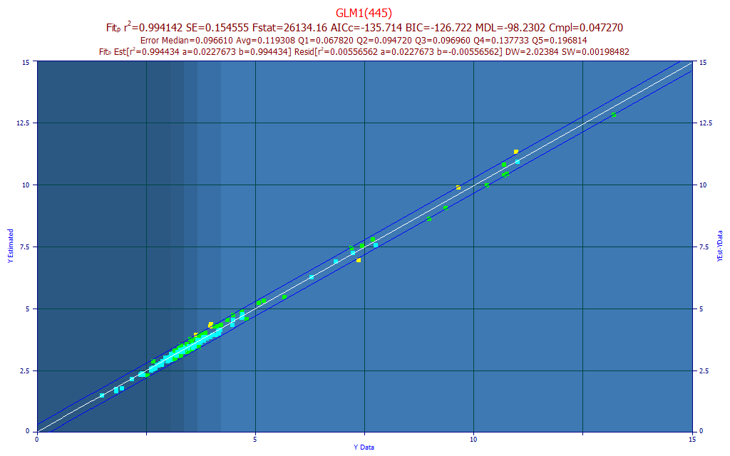
Fig 11. Model plot for 445 nm single predictor total curcuminoids UV-VIS model

In the model plot shown in Fig. 11, the chromatography reference values are on the X-axis and the predicted values are on the Y-axis. These are Y-known (chromatography) vs. Y-estimated (spectroscopy model) plots. If you find yourself content with this measure of predictive accuracy, you are in agreement with the F-statistic and MDL metrics, that a single predictor UV-VIS model suffices for total curcuminoids.

The 445 nm predictor fits with the 448 nm peak in the Fig. 7a peak fit and the 446 nm peak in the Fig. 7b peak fit. This 445 nm model produced a 0.0966 median prediction error where the 425 nm predictor model (a reasonable curcuminoid central wavelength) produced a 0.1040 median prediction error - the 445 nm model is a better predictor of total curcuminoids.

PLS vs Direct Spectral Modeling of this UV-VIS Data Matrix

The statistics for the 445 nm direct spectral fit model are follows:

Prediction Statistics - from Original Fit - Leave One Out

   r²       SE       F-stat       AICc       BIC       MDL       DOF

0.9941419      0.1545550      2.613e+04      -135.7143      -126.7226      -98.23023       154

 Median Err       Avg Err       Avg Err Q1       Avg Err Q2       Avg Err Q3       Avg Err Q4       Avg Err Q5

0.0966062      0.1193078      0.0678179      0.0947165      0.0969568      0.1377332      0.1968144

 Quintile       Lower       Upper

  First      1.4797533      3.0649067

  Second      3.0649067      3.3511367

  Third      3.3511367      3.6682000

  Fourth      3.6682000      4.1988067

  Fifth      4.1988067      13.198050

Parameter Statistics

 Parm      Value      Std Error      t-value      95%ConfLo      95%ConfHi      P>|t|

Constant      -0.04954104      0.027720924      -1.78713536      -0.10430340      0.005221311      0.07588

    445      0.011068653      6.67272e-05      165.8790627      0.010936834      0.011200472      0.00000

Data      Yobserved      Ypredict      Residual      ResStnd      *      ID

157      4.0907035      4.0907035      -1.45e-10      -9.71e-10            Average

Fig 12. Fit statistics for 445 nm single predictor total curcuminoids UV-VIS model

The r² of prediction, 'leave one out', is 0.99414. This corresponds with 5858 ppm statistical (normalized sum of squares) error.

Partial Least Squares (PLS) is often used for mathematically modeling spectra. We will now contrast this very simple 1 predictor (2-parameter) direct spectral fit model with PLS models built using this same data matrix. To do this, we used Systat's NIPALS implementation of PLS, the same 5 nm wavelength predictor spacing, and the same leave one out prediction statistics. The PLS algorithm is a complex statistical procedure which fits factors or latent variables generated from successive correlations. It produces a model with as many coefficients as there are wavelengths (plus one more if a constant is fitted). In the PLS fits shown below, there are 33 coefficients for each wavelength and 34 parameters total:

Fig 13. PLS NIPALS models for total curcuminoids UV-VIS data matrix

In the table shown in Fig. 13, we averaged all 156 of the spectra at each wavelength (column 1). This is the average of all spectra shown in Fig 8. The average of 156 total curcuminoid Y values is the 4.09 at the bottom of column 1. We then multiplied the estimated coefficients from each PLS fit (factors 1-8) by the average spectrum and these are the values shown in columns 3-10. The r² of prediction (leave one out) is in the heading (second row) for the factors 1 through 8 fits. The best r² of prediction occurs with 3 factors.

Our very simple 1 predictor (2-parameter) linear direct spectral fit model has an r² of prediction of 0.99414 (5,858 ppm), slightly better than the 0.99374 (6,257 ppm) of the 3-factor PLS, and appreciably better than the PLS 1-factor model (12,998 ppm).

We also ran Unscrambler's NIPALS PLS with the leave one out prediction errors. In its modeling, we saw a slightly better PLS performance using a 1 nm spacing (161 parameters) - it optimized to four factors with an r² of prediction of 0.99392 (6,083 ppm). We also fit Unscrambler's PCR (principal component regression) algorithm; it's best prediction performance occurred with five principal components and an r² of prediction of 0.99389 (6,110 ppm).

In looking at each of the PLS columns above, you see the influence at each WL, the actual value, positive or negative, that sums into the overall estimate. The 1-factor PLS gives very nearly the same weight to each WL, and all are positively correlated. The differences begin to appear as the factor count increases. The three factor model, having the lowest prediction errors, does find the 445 nm predictor (highlighted in red) to be strongest, though only slightly so. All of the 355-480 nm predictors add to the overall prediction estimate, the 320-350 nm predictors subtract from it.

It may be instructive to compare the full permutation direct spectral fits in this same manner. Here the specific model selected for each predictor count was that one most compliant in WLs with all of the retained models of that count (in our case, 100 models each). For each predictor count, we are thus seeing the one model best representing the wavelengths most consistently appearing in the retained models, not that model furnishing the best estimated prediction.

Fig 14. Full permutation direct spectral fits for total curcuminoids UV-VIS data matrix, most WL compliant model at each predictor count

If you look closely at the direct spectral data in Fig 14, you will see that there is a convergence to specific WLs as the predictor count increases and there are also many WLs that do not appear in any of these models.

In our Gaussian peak fit of the average turmeric spectrum (Fig. 7a) we saw 336, 356, 377, 398, 418, 433, 448, and 466 nm wavelengths.

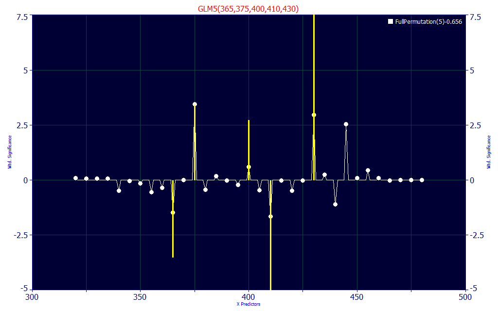
Fig 15. Significance vs WL map for all retained 5-predictor full permutation direct spectral fits

Fig 15 contains a significance map where the wavelengths for the best 100 retained 5-predictor models are shown in the white curve. Here we see all but one of these eight wavelengths represented. The four highest amplitude peaks: 398, 418, 433, and 448 nm are strongly represented in the significance map.

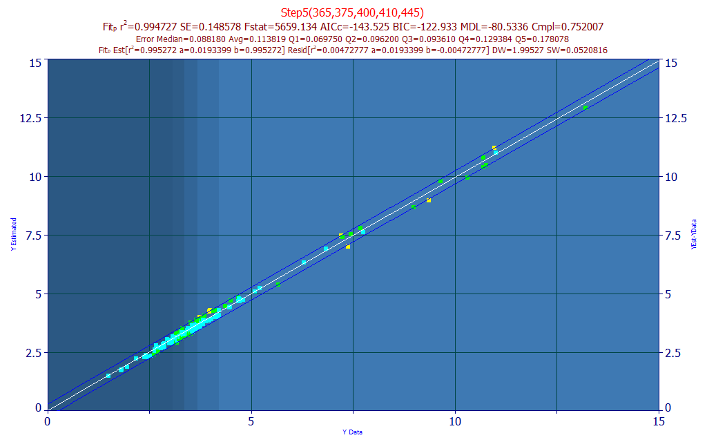
Fig 16. Model plot for 365-375-400-410-445 nm five predictor total curcuminoids UV-VIS model

This highest compliance five parameter model shown in Fig. 16 has 365, 375, 400, 410, and 445 predictors. This five-predictor model offers an r² of 0.9947, a small improvement over the single predictor's 0.9941. When looking at r² values, you must look at the 1-r² that represents the normalized statistical (sum of squares) error. In this instance, the 1 predictor model has an error of 5860 ppm, this five predictor model an error of 5270 ppm. If we look at the average error, we have 0.1193 on the one predictor model vs. 0.1138 on the five parameter model. This is even more pronounced in the highest quintile of total curcuminoids (4.2-13.2%) where the error drops from 0.1968 to 0.1781 with the five parameter model.

Higher Predictor Count Total Curcuminoids Model

Random sampling prediction errors can be used instead of leave one out prediction errors when you cannot assume that you have fully bracketed the modeling problem and out of nowhere a sample may appear outside the properties of all samples used in the modeling. In a random sampling error estimation, random in-sample and out-of-sample sets, both usually of a fair size, are used, the former to generate the models and the latter to evaluate blind predictions. It is assumed that some count of the data sets defining the bracketing of the modeling problem will randomly appear in the out-of-sample set, and thus the models formed from the in-sample sets will be incomplete. Should you use random sampling errors, we can recommend a 2/3 size for the in-sample model set, and a 1/3 size for the out-of-sample test set. When using random sampling for prediction error information, you can specify average errors, or the maximum worst-case errors, from amongst the count of test instances.

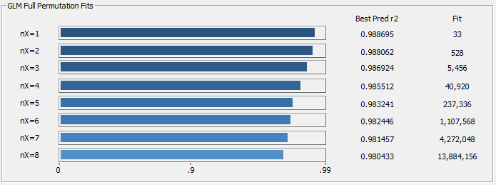
Fig 17a. r² averages of the ten best retained models for each predictor count using worst case errors in a 2/3, 1/3 random sampling

In the Fig. 17a progress display of the average of ten best retained fits at each predictor count in the full permutation fitting, the r² of prediction comes from the worst-case random sampling errors with 100 random sets of 104 in-sample spectra, and 52 out-of-sample spectra, and only the worst error of the 100 random sets is reported. As you will note, the higher the predictor count, the higher the likelihood of seeing predictions lose accuracy as a result of an incomplete bracketing of the modeling problem.

Fig 17b. r² averages of the ten best retained models for each predictor count using average errors in a 2/3, 1/3 random sampling

The worst case prediction errors are useful in critical applications. When average random sampling errors are used, as shown in Fig. 17b, there is no observable penalty with predictor count for this data matrix. This means the bracketing has a considerable measure or redundancy. This is the value of having a comprehensive library of modeling spectra. It does mean that a design of experiments, or the acquisition of a wide representation of commercial samples, are necessary for truly stable and effective predictive models.

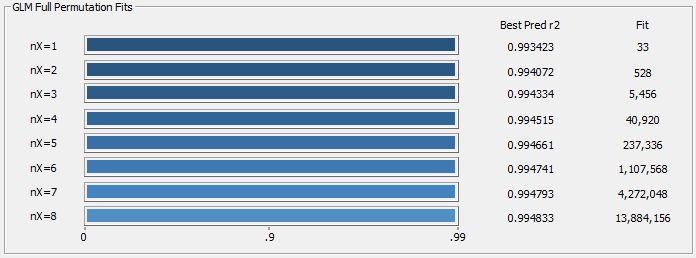
Fig 17c. Averages of the ten best retained models for each predictor count using 'leave one out' prediction errors

In Fig. 17c, we see the averages of the 10 best retained models for each predictor count for Leave One Out prediction errors. In general, if the data matrix consists of a well-crafted library, the leave-one-out errors will have only a slightly better prediction errors, as shown here. A Leave One Out procedure is the equivalent of a random sampling with N discrete pairs of in-sample data of size N-1 and out-of-sample data of size 1.

Direct Spectral Fit of BDMC

We now shift to a more challenging modeling problem. To fit the BDMC component amount in turmeric, the modeling algorithm must sort the BDMC spectral information from all other curcuminoid information. That will be more difficult given that the three principal curcuminoids all have close to the same UV-VIS absorbance.

We also acknowledge that the 'BDMC' estimate will also consist of a second much smaller curcuminoid component that elutes in the shoulder of the BDMC peak, and which the chromatography was generally unable to separate. We thus fit not just the amount of BDMC, but also this smaller amount of elution companion curcuminoid.

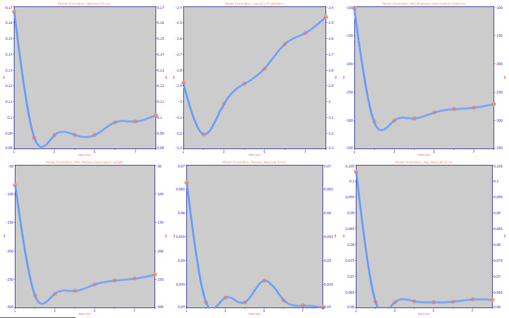
Fig 18. The performance metrics for the full permutation BDMC UV-VIS modeling

If we do the same kind of optimization for the BDMC model that we did for the total curcuminoids model, Fig. 18, we see a much more consistent behavior. Every metric shows the optimum to be 2-3 predictors, and most slightly favor the 2. We would expect the 1-predictor models to be poor, incapable of separating the different curcuminoids, and that is confirmed in the performance plots.

Fit Statistics

   r²       SE       F-stat       AICc       BIC       MDL       DOF

0.9597554      0.0819304      1824.3768      -332.6438      -320.7093      -296.7209       153

Prediction Statistics - from Original Fit - Leave One Out

   r²       SE       F-stat       AICc       BIC       MDL       DOF

0.9548470      0.0867830      1617.7379      -314.6910      -302.7565      -279.2489       153

 Median Err       Avg Err       Avg Err Q1       Avg Err Q2       Avg Err Q3       Avg Err Q4       Avg Err Q5

0.0439206      0.0609729      0.0385567      0.0481725      0.0448016      0.0536304      0.1178679

 Quintile       Lower       Upper

  First      0.2888600      0.5105413

  Second      0.5105413      0.5969833

  Third      0.5969833      0.6925670

  Fourth      0.6925670      0.8138550

  Fifth      0.8138550      2.2839867

Parameter Statistics

 Parm      Value      Std Error      t-value      95%ConfLo      95%ConfHi      P>|t|

Constant      0.024483141      0.015090018      1.622472670      -0.00532855      0.054294834      0.10676

    415      0.016762818      0.000586221      28.59469669      0.015604685      0.017920950      0.00000

    450      -0.02013094      0.000781259      -25.7673158      -0.02167439      -0.01858750      0.00000

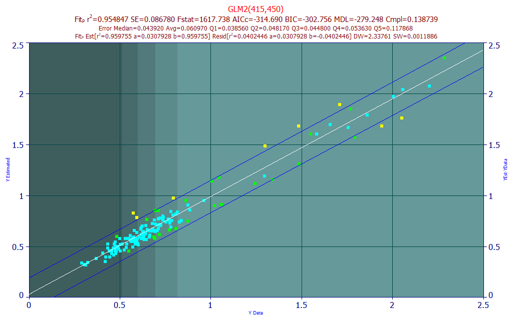
Fig 19. Model plot and prediction statistics for 415,450 nm two-predictor BDMC UV-VIS model

The best 2-predictor model shown in Fig. 19 has a much lower r² than the total curcuminoid model, 0.9548 (45,200 ppm error). The average errors are lower, 0.0610, in absolute terms, but the BDMC only ranges up to 2.5% of the turmeric (where the total curcuminoids in the model data go up to 13%). The BDMC model errors are appreciably wider, as shown in the model plot.

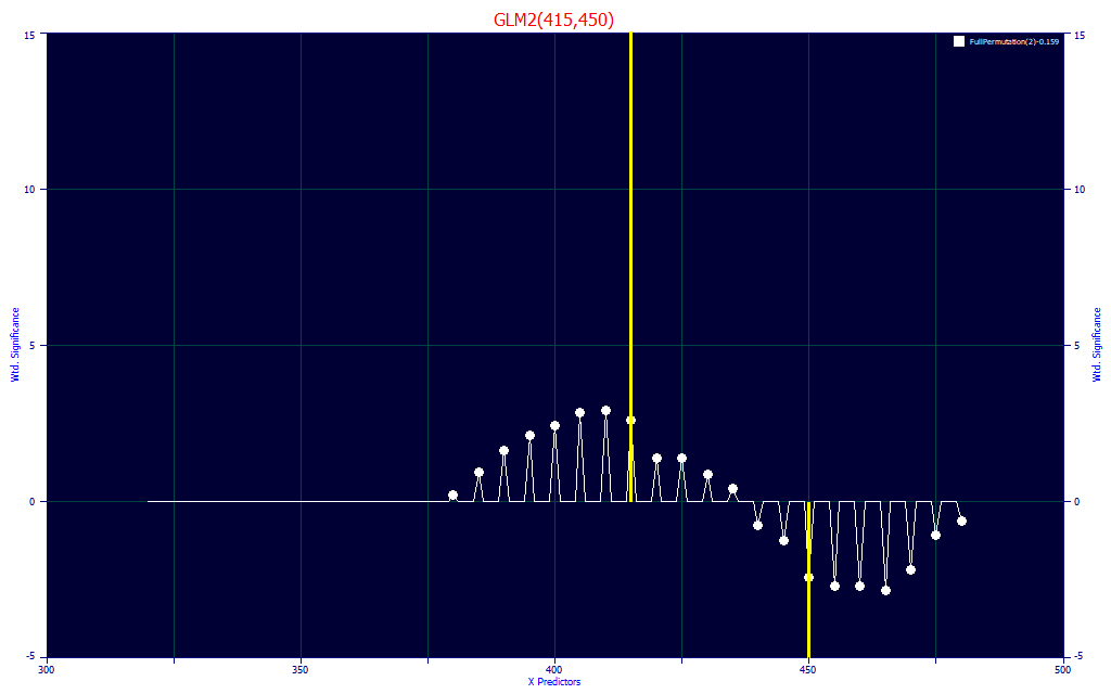
Fig 20. Significance vs WL map for all retained 2-predictor full permutation direct spectral fits of BDMC data

In Fig. 20, we look at this specific 2-predictor BDMC model on a WL map that shows the statistical significance of the different WLs for the retained fits (here the 100 best retained fits with 2-predictors), we see no models with a UV wavelength up to 375 nm, despite there being a significant difference between the BDMC and the other curcuminoids in the UV. That may be associated with this unknown BDMC companion peak which varies significantly sample to sample and has a higher UV absorbance than the three principal curcuminoids (Fig. 5). In this 2-predictor model, the BDMC is estimated from its central WL, and the 450 nm signal (where BDMC falls off faster than all of the other curcuminoids) furnishes the subtraction of the other curcuminoids.

When fitting components in natural products where there may be a strong correlation with the total of a given class of compound, it is recommended that you check the correlations. The correlation between the BDMC and total curcuminoids is such that an r²>.7655 is needed for a model to be better than a BDMC average fraction from all data sets used as a scalar of the estimated total curcuminoids. Although the BDMC fit is weaker than the total curcuminoid fit, it easily improves upon this correlation.

Systat PLS NIPALS fits, 5 nm intervals, optimized to 4 factors with a leave one out r² of prediction of 0.9462 (53,840 ppm error). Unscrambler PLS NIPALS fits, processing every nm instead of every 5 nm, 161 wavelengths, fared better, the best prediction with 3 factors and a leave one out r² of prediction of 0.95347 (46,530 ppm error). Unscrambler PCR, again every nm, had the best prediction with 3 principal components and a leave one out r² of prediction of 0.95352 (46,480 ppm error). Although the PLS and PCR models were nearly as good as the direct spectral fit selected above, note that this far simpler 3-coefficient direct spectral fit still outperformed the best 162-coefficient PLS and PCR models.

Direct Spectral Fit of Curcumin

We would expect to fare better with a curcumin component model since there is no coeluting chromatographic component to muddy the waters, and in nearly all turmeric samples, the curcumin has the largest presence within the three principal curcuminoids. Indeed, we see models with very close to the same performance as observed with the total curcuminoids and about the same ambiguity amongst the optimization statistics.

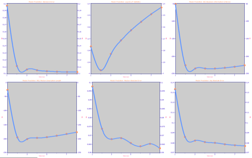
Fig 21. The performance metrics for the full permutation Curcumin UV-VIS modeling

If we look at the performance metrics in Fig. 21, we once again see the r² and the median and absolute errors at the 6-8 predictors. As before, we favor the BIC and MDL, both of which suggest the optimum to be 3 predictors.

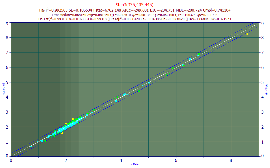
Fig 22. Model plot for 335,405,445 nm three predictor curcumin UV-VIS model

This three predictor curcumin model, Fig. 22, offers a 0.9925 r² of prediction (7,437 ppm error) and a 0.082 average error on curcumin values that can be as high as 8% of the turmeric.

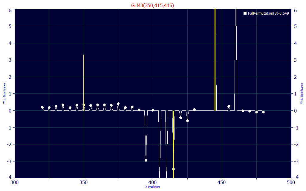
Fig 23. Significance vs WL map for all retained 3-predictor full permutation direct spectral fits of Curcumin data

The wavelength significance map for the best retained 3-predictor models shown in Fig.23 uses a UV WL (it seems almost any will do), and a high visible WL, to estimate the curcumin, and values left of the curcumin central peak to estimate the subtraction of the other curcuminoids.

The correlation between the curcumin and total curcuminoids is quite high. An r²>.9633 is needed for the model to be better than a curcumin average fraction scalar of the estimated total curcuminoids. Here, as with the BDMC, the curcumin fit's r² of .9925 easily improves upon this correlation.

Systat PLS NIPALS fits, 5 nm intervals, optimized to 5 factors with a leave one out r² of prediction of 0.9917 (8,302 ppm error). Unscrambler PLS NIPALS fits, processing every nm instead of every 5 nm, 161 wavelengths, was slightly better, the best prediction with 4 factors and a leave one out r² of prediction of 0.99199 (8,010 ppm error). Unscrambler PCR, again every nm, had the best prediction with 5 principal components and a leave one out r² of prediction of 0.99209 (7,910 ppm error). Again we note that the PLS and PCR models performed well, but we realized 7437 ppm in a very simple 4-coefficient, 3-wavelength direct spectral fit.

Direct Spectral Fit of DMC

Here we expect difficulties to arise. Sandwiched between the BDMC and C spectrally (Fig. 4 and Fig. 5), there are almost no WLs where the DMC is either the highest or lowest signal amongst the three principal curcuminoids. Also, the DMC, like the curcumin, is strongly correlated with the total curcuminoids. For a DMC model to improve upon an average DMC fraction of the total estimated curcuminoids, the r² must be >.9604 (39,600 ppm).

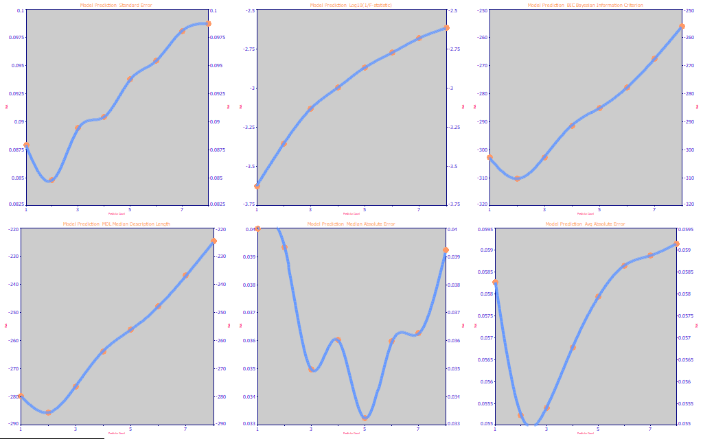
Fig 24. The performance metrics for the full permutation DMC UV-VIS modeling

In Fig. 24, we see that the DMC model fitting optimizes reasonably well to 2 predictors.

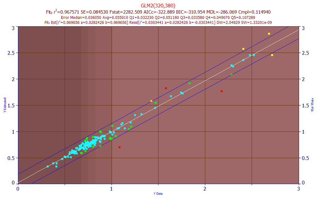
Fig 25. Model plot for 320,380 nm two predictor DMC UV-VIS model

The model plot is shown in Fig. 25. The r² of prediction of the best 2-predictor model, 0.9675 (32,500 ppm), is only marginally better than a DMC estimate based on the average fraction of DMC across all samples times the estimate of total curcuminoids.

Here, a simple design consideration would be to estimate the total curcuminoids, the BDMC, and the curcumin, and to report the DMC as the difference between the two estimated components and the total. The DMC, narrowly tucked between the BDMC and curcumin spectrally, is respectably fitted, but only in the UV, and as far as the modeling goes, there is little difference between fitting the DMC from the chromatography and estimating the total curcuminoids and multiplying that value by the average DMC fraction across all of the samples.

We also note the apparent outliers (>3SE), the points colored in red, are not true data outliers. One of these has BDMC>DMC (rare), another has DMC>curcumin (rare), and another has very close to the highest curcumin fraction of curcuminoids in the data matrix. Unlike the other models that managed these spectra representing bounds in the data, this DMC model fails.

The PLS fits for this data optimized to 3 factors with a leave one out r² of prediction of 0.9642 (35,800 ppm error).

Systat PLS NIPALS fits, 5 nm intervals, optimized to 3 factors with a leave one out r² of prediction of 0.9642 (35,800 ppm error). Unscrambler PLS NIPALS fits, processing every nm instead of every 5 nm, 161 wavelengths, was similar, the best prediction with 3 factors and a leave one out r² of prediction of 0.96406 (35,940 ppm error). Unscrambler PCR, again every nm, had the best prediction with 3 principal components and a leave one out r² of prediction of 0.96403 (35,970 ppm error). Here again, the simple direct spectral fit's error (32,500 ppm) is better and achieved with just 2 wavelengths (3 parameters).

The UV-VIS Modeling Methodology using the Chromatography's Spectral Data

In this white paper, we sought to illustrate the value of using the chromatography's own 3D spectral data to extract UV-VIS data sufficient to explore the viability of UV-VIS direct spectral modeling. When the chromatographic data are saved in this 3D format, the evaluation of UV-VIS spectral models based on that chromatography becomes a software task. No laboratory spectra need be run that were not already run with the chromatography. The evaluation shown in this white paper can be accomplished in hours as opposed to days or weeks.

Although this white paper has illustrated rather straightforward UV-VIS models, we should note that many turmeric spectral models, particularly in the NIR, require considerably higher predictor counts. These NIR models are covered in Modeling Spectra - Part II - FTNIR Data.