PeakLab v1 Documentation Contents            AIST Software Home            AIST Software Support

Modeling Spectra - Part II - FTNIR Data

Authors: Amruta Behera¹ (amruta.behera@plaksha.edu.in), Hasika Suresh² (hasika.suresh@tufts.edu), Rudra Pratap³ (rudra.pratap@plaksha.edu.in), Ron Brown⁴ (ron@aistsoftware.com)
Publish Date: January 2023.

¹Amruta Behera is a founding professor at the new Plaksha University in Mohali, the planned city in the Punjab near Chandigarh, India. Amruta managed the project where the data shown in this white paper was generated as part of his several years of post-doctoral research at the Indian Institute of Science (IISc) in Bangalore, India. In this project, handheld spectrometers were designed, built, and tested for in-field analysis of spices and other cultivated botanicals.

²Hasika Suresh is a doctoral student in the department of Chemical and Biological Engineering at Tufts University, Boston. While she was at the Centre for Nanoscience and Engineering (CeNSE) at IISc India, she developed the HPLC methodology for curcuminoid and turmeric samples and worked to procure a vast library of turmeric roots and powders. Hasika generated all of the chromatographic data illustrated in this white paper.

³Rudra Pratap is the founding vice chancellor (president) of Plaksha University. Prior to this position, Rudra served as the Deputy Director of Indian Institute of Science, Bangalore, India where he founded of the IISc Centre for Nano Science and Engineering (CeNSE) and where, for a time, he served as chairman of the board of a major scientific and statistical software company. In an effort to create tools for Indian farmers growing spice crops to better quantify the value of their harvests, Rudra created and guided the R&D project that resulted in all of the chromatographic and spectroscopic data that appears in this series of modeling white papers. The samples analyzed in these white papers were collected across several years and now represent what we believe to be the most comprehensive and diverse library of commercially grown turmeric in the world.

⁴Ron Brown is the founder of AIST Software, in Oregon, USA, and the author of the PeakLab software, as yet unreleased, which was used to analyze much of this data that appears in these white papers. Ron developed the original PeakFit software and also authored the TableCurve software products for curve and surface fitting as well as AutoSignal for signal analysis.

FTNIR Spectral Modeling

In this white paper, we will demonstrate FTNIR spectral modeling in an example where we estimate the total curcuminoids and the three principal curcuminoid components in turmeric powders.

You may wish to review the Modeling Spectra - Part I - UV-VIS Data white paper prior to this one. It illustrates many of the basics associated with modeling curcuminoids in the context of liquid spectra derived from UV-VIS data reconstructed from the diode array detector of the chromatography.

In that which follows, we will fit the same chromatographic values for the turmeric powders as in Part I, but instead of using liquid UV-VIS spectra, we will use powder FTNIR spectra. By directly analyzing the powders, we will see a much more complex modeling problem. The absorbance of powders is impacted by both powder particle size and powder moisture levels. The particle size density will vary across the turmeric samples as a consequence of processing, and the NIR spectra for a given turmeric will vary with the moisture (there are two prominent water bands in the NIR).

HPLC method

An Agilent 1260 Infinity II series chromatograph was used with Infinity Lab Poroshell 120 EC C-18 UHPLC column, 4.6*50 mm, 2.7 micron, to produce the separation of the curcuminoids. The separations were isocratic using a mobile phase of 0.2% orthophosphoric acid:Acetonitrile at a 55:45 (v/v) ratio. The separations were carried out at a flow rate of 0.8ml/min, a temperature of 40C. and injection volume of 20 ”l. Concentrations and run time varied depending on the materials and the objectives of the separations. For most runs, the three principal curcuminoids would elute between 2.5-4.5 minutes. The spectra were read at 425 nm. As described in Part I, a small amount of curcuminoid coeluting with the BDMC is included in the BDMC measurement, and for aromatic turmeric, a curcuminoid coeluting with DMC is similarly included in the DMC measurement.

FTNIR method

A Perkin-Elmer Spectrum Two N FTNIR Spectrometer was furnished by Perkin Elmer to authors 2 and 3 for the analysis of their turmeric library. The NIR Reflectance module was used for these analyses of the raw turmeric powders, and five replicates were run for each sample. We thank Perkin Elmer India Pvt Ltd for their kind support of the handheld turmeric analysis project initiative.

FTNIR Spectroscopy of Curcumin - 1600-1850 nm WL Band

When dealing with the spectra of a natural product, such as the turmeric in this example, we first look at the target components, the curcuminoids, in FTNIR spectra. We then look at the natural material, the turmeric powders, to see how cleanly the target spectrum appears. We want to know whether that target spectrum is distorted or obfuscated by additional non-target components that happen to have absorbances in the same modeling band.

This isolation of the target spectrum was simple for the US-VIS of curcuminoids in turmeric. Nearly all of the 320-480 nm UV-VIS modeling band signal consisted of just the target components. That is not the case in the NIR. Further, the analysis of powders instead of solvent extracts of those powders means we will be measuring a reflectance rather than a transmission spectrum, with all of the additional complications of the optics of powders.

We begin with the baseline-corrected peak fit of FTNIR spectra for a mixed-curcuminoid standard that is 80% curcumin, 17% DMC (demethoxycurcumin) and 3% BDMC (bis-demethoxycurcumin), and which has a minimum 95% total curcuminoid purity.

Fitted Parameters

r² Coef Det      DF Adj r²      Fit Std Err      F-value      ppm uVar

0.99998832      0.99998714      0.00060991      865,362      11.6841106

 Peak      Type       a₀       a₁       a₂

    1      Gauss      0.07754611      1622.94995      3.62585906

    2      Gauss      0.19156402      1631.38090      3.62585906

    3      Gauss      0.58525963      1638.12025      3.62585906

    4      Gauss      0.93053074      1645.32838      3.62585906

    5      Gauss      1.37703622      1652.16889      3.62585906

    6      Gauss      1.16158109      1658.94666      3.62585906

    7      Gauss      1.94094160      1664.80261      3.62585906

    8      Gauss      4.86791430      1671.85663      3.62585906

    9      Gauss      3.17056598      1678.65920      3.62585906

   10      Gauss      3.65678293      1685.21028      3.62585906

   11      Gauss      2.84097192      1691.73025      3.62585906

   12      Gauss      2.12277520      1697.74234      3.62585906

   13      Gauss      1.57268002      1703.92320      3.62585906

   14      Gauss      1.20276297      1709.41814      3.62585906

   15      Gauss      1.22046158      1715.43078      3.62585906

   16      Gauss      1.11518039      1721.28791      3.62585906

   17      Gauss      0.53211531      1727.83422      3.62585906

   18      Gauss      0.37295564      1733.90366      3.62585906

   19      Gauss      0.48643820      1741.44409      3.62585906

   20      Gauss      0.10314512      1752.02710      3.62585906

   21      Gauss      0.07910649      1770.44331      3.62585906

   22      Gauss      0.10023469      1778.12429      3.62585906

   23      Gauss      0.44778885      1785.94190      3.62585906

   24      Gauss      0.32272304      1791.96287      3.62585906

   25      Gauss      0.10306116      1798.20288      3.62585906

   26      Gauss      0.09156754      1807.08403      3.62585906

   27      Gauss      0.01106229      1818.11011      3.62585906

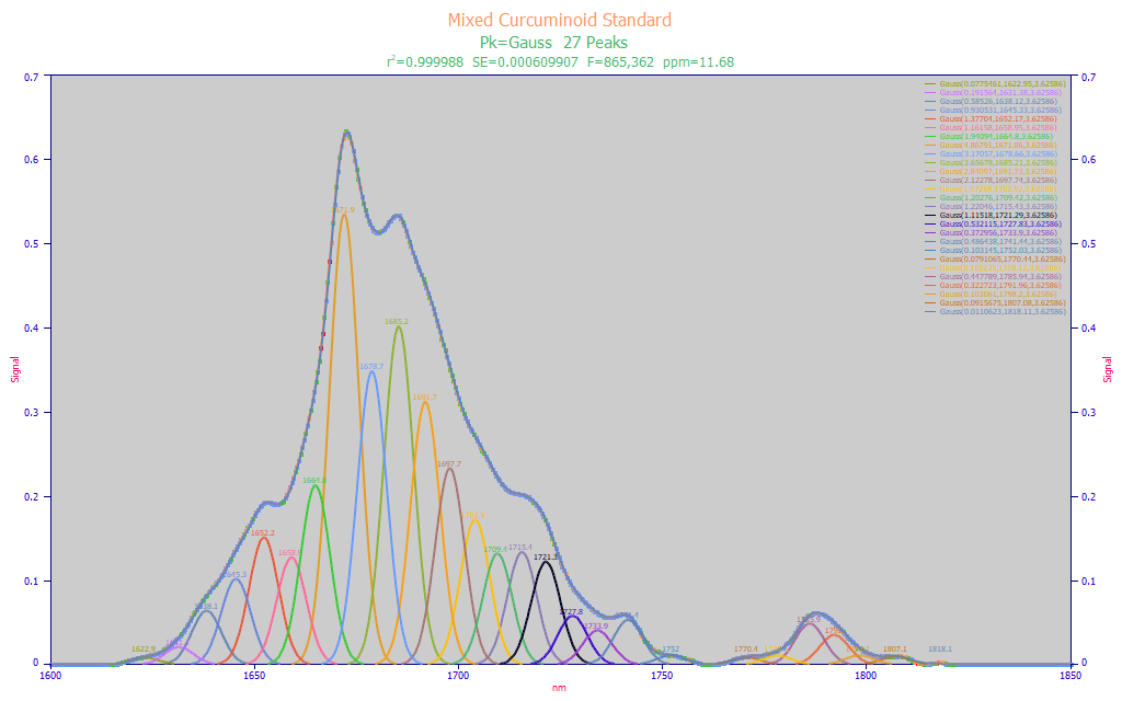
Fig. 1 Constant-width multiple Gaussian fit to baseline-corrected FTNIR wavelength spectra for mixed curcuminoid standard, 1600-1850 nm

The NIR spectral information between 1600 and 1850 nm is often used for curcuminoid modeling. Although we fit constant width Gaussians, and wavelength instead of frequency spectra, we realized a 11.7 ppm statistical error, and an F-statistic of 865K, in fitting 27 Gaussian peaks to this spectral data. The shared width of the 27 peaks in the fitting is 3.63 nm. While this count of Gaussians may seem excessive, FTNIR has superb resolution and the four peaks that make up the central portion of the spectral feature correspond beautifully to the unusual spectral shape at the peak. We feel it highly likely that the spectral data really does have a Gaussian SD width (a₂) of less than 4 nm. As a comparison, we saw 12 nm UV-VIS Gaussian SD widths in Part I.

Peak modeling of NIR spectra can be a complex task, and that is all the more so with FTNIR data where the resolution of the instrument is a good deal better than non-Fourier NIR spectrometers.

We fit the spectral data to Gaussians to determine the approximate width of the spectral peaks being resolved by the spectrometer, and also to get a sense for the spectral WLs likely to be seen in a direct spectral fit. With a Gaussian SD width of 3.63 nm (a FWHM of 8.5 nm and a 10% amplitude full width of 17.1 nm), we can apply the rule of thumb we discussed in Part I where we use approximately half the Gaussian SD, here a 2 nm spacing, for the actual spectral modeling. With respect to approximate wavelengths we would likely see in a direct spectra model fit, there is curcuminoid absorbance everywhere in the band, although we will note that the 1672, 1678, 1686, and 1692 are the four principal WLs we would expect to appear in FTNIR 2 nm-spaced models. We also take note of the 1786 nm peak which stands apart.

FTNIR Spectroscopy of Turmeric - 1600-1850 nm WL Band

Fitted Parameters

r² Coef Det      DF Adj r²      Fit Std Err      F-value      ppm uVar

0.99999879      0.99999858      0.00016186      4,860,878      1.21306151

 Peak      Type       a₀       a₁       a₂

    1      Gauss      0.21293555      1667.52760      4.00639983

    2      Gauss      0.45704880      1673.80813      4.00639983

    3      Gauss      0.74660610      1680.79754      4.00639983

    4      Gauss      1.10956919      1687.38247      4.00639983

    5      Gauss      1.64452145      1693.40032      4.00639983

    6      Gauss      1.87616269      1699.63660      4.00639983

    7      Gauss      1.86457862      1705.79046      4.00639983

    8      Gauss      1.76489039      1711.98395      4.00639983

    9      Gauss      1.59420368      1718.43736      4.00639983

   10      Gauss      1.62444512      1724.68704      4.00639983

   11      Gauss      1.77634726      1731.01182      4.00639983

   12      Gauss      1.82518989      1737.34139      4.00639983

   13      Gauss      1.96161935      1743.50345      4.00639983

   14      Gauss      2.14083500      1749.65760      4.00639983

   15      Gauss      2.16663371      1755.70319      4.00639983

   16      Gauss      2.08492862      1761.71595      4.00639983

   17      Gauss      2.07783384      1767.59397      4.00639983

   18      Gauss      2.18217731      1773.56989      4.00639983

   19      Gauss      2.22647553      1779.62857      4.00639983

   20      Gauss      2.02101737      1785.60858      4.00639983

   21      Gauss      1.77858801      1791.67217      4.00639983

   22      Gauss      1.50039661      1797.61488      4.00639983

   23      Gauss      1.28210730      1803.52385      4.00639983

   24      Gauss      1.10044513      1809.52124      4.00639983

   25      Gauss      0.98591395      1815.63993      4.00639983

   26      Gauss      0.88743719      1821.93406      4.00639983

   27      Gauss      0.71785622      1828.35192      4.00639983

   28      Gauss      0.46847552      1834.94017      4.00639983

   29      Gauss      0.17950584      1841.68676      4.00639983

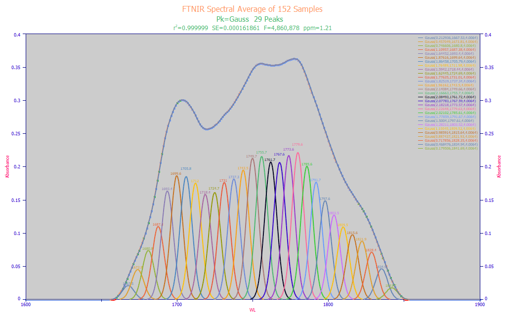
Fig. 2 Constant-width multiple Gaussian fit to baseline-corrected FTNIR wavelength spectra for an average spectrum from 152 turmeric samples, 1600-1850 nm

Clearly the natural material spectrum fitted in Fig. 2 looks drastically different from the approximate target spectrum in Fig. 1. The turmeric 1600-1650 nm spectral information melds the initial curcuminoid Gaussian peaks into its elevated absorbance baseline signal. A proper modeling band thus begins at about 1650 nm and the turmeric absorbances begin to meld into the water band at about 1850 nm.

The turmeric spectrum is an average of 152 distinct turmeric samples, each an average of 5 FTNIR spectra replicates. The average of the known % total curcuminoids was 3.869% (the value we would expect to see from any predictive model that processed this composite spectrum). This averaged spectra's close to optimal fit has virtually everything prominent between 1690-1790 nm, and a shared a₂ width of 4.00 nm. We do see a superb 1.2 ppm statistical error of fit with 29 Gaussian peaks of equal width.

We know the instrument's resolution will not change whether one is looking at a three-component standard, or a natural material with over a hundred documented components, and here, the optimum peak fit (by F-statistic) does produce a width that is reasonably close to the target material.

The spectra of the target spectrum within the natural material did get seriously obfuscated with additional spectral content. Assuming the NIR target curcuminoid wavelengths do not significantly change in a curcuminoid reference powder versus that of the natural turmeric powder, we must assume that there is a good measure of non-curcuminoid absorbance in the modeling band. The curcuminoid mixed standard has only a small spectral feature beyond 1750 nm, but the turmeric spectra has its maximum in this region and easily half of the signal which would be exposed to the modeling algorithm.

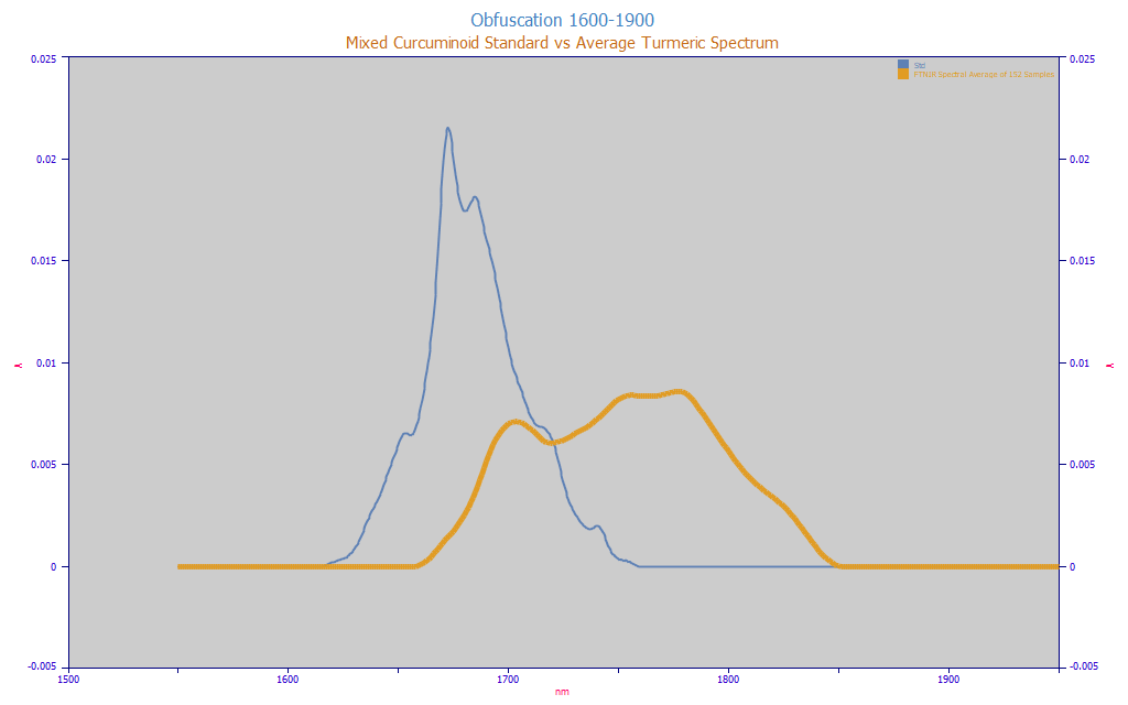
Fig. 3 Obfuscation of Curcuminoid Target Spectrum in Natural Turmeric (average spectrum from 152 turmeric samples), 1600-1850 nm, Equal Area

In Fig. 3, we plot the obfuscation, the extent to which the target spectrum the modeling must identify matches the spectrum of the natural material.

We also acknowledge the possibility that the hydrophobic oils, turmerones, and other high MW compounds in the turmeric powders might act as solvents of sorts and the above plot also represents spectral shifts in the curcuminoid signal. If so, we would expect the information from 1725-1800 in the amber curve to be positively correlated with the amount of total curcuminoids. We would expect non-curcuminoid signal to be negatively correlated.

FTNIR Spectroscopy of Curcumin - 2100-2300 nm WL Band

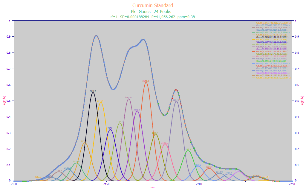
The 2100-2300 nm band is likewise used for curcuminoid modeling and was generally preferred by a number of authors for furnishing better modeling of both total curcuminoid and the individual curcuminoid principal components. The general premise is that the curcumin, the demethoxycurcumin (DMC) and bis-demethoxycurcumin (BDMC) have more strongly unique NIR signatures in this band. We perform a multiple-Gaussian fit to a pure curcumin standard where only curcumin is detected in the chromatography:

Fitted Parameters

r² Coef Det      DF Adj r²      Fit Std Err      F-value      ppm uVar

0.99999962      0.99999959      0.00018828      41,056,262      0.38159004

 Peak      Type       a0       a1       a2

    1      Gauss      0.04777814      2113.23907      3.26660685

    2      Gauss      0.20069334      2119.63324      3.26660685

    3      Gauss      0.48343107      2124.19170      3.26660685

    4      Gauss      0.61595751      2129.09761      3.26660685

    5      Gauss      0.92922934      2133.64488      3.26660685

    6      Gauss      1.96529681      2138.23145      3.26660685

    7      Gauss      4.52609082      2142.64396      3.26660685

    8      Gauss      4.02386680      2146.90359      3.26660685

    9      Gauss      2.63591702      2151.98579      3.26660685

   10      Gauss      2.97545901      2157.10426      3.26660685

   11      Gauss      4.20290436      2161.88348      3.26660685

   12      Gauss      3.58633907      2166.47597      3.26660685

   13      Gauss      5.04049258      2171.26439      3.26660685

   14      Gauss      2.39782482      2176.41680      3.26660685

   15      Gauss      1.89720807      2181.49756      3.26660685

   16      Gauss      4.08101164      2187.60137      3.26660685

   17      Gauss      1.55759640      2193.89666      3.26660685

   18      Gauss      0.76871206      2199.23269      3.26660685

   19      Gauss      0.65406307      2205.33283      3.26660685

   20      Gauss      0.40569784      2210.90152      3.26660685

   21      Gauss      0.36877495      2215.79566      3.26660685

   22      Gauss      0.48384132      2221.21627      3.26660685

   23      Gauss      0.22801481      2230.84438      3.26660685

   24      Gauss      0.03200831      2235.83215      3.26660685   

Fig. 4 Constant-width multiple Gaussian fit to baseline-corrected FTNIR wavelength spectra for pure curcumin, 2100-2250 nm

The fit shown in Fig. 4 covers the 2100-2250 nm band and requires 24 Gaussians produce an outstanding 0.38 ppm statistical error in an F-statistic peak fit optimization. The fitted widths are somewhat less, 3.27 nm versus the 3.62 nm we saw for the 1650-1850 band. That might possibly be expected; line broadening in spectra would be a mix of a fixed Gaussian IRF (instrument response function) and a Lorentzian (natural spectral line broadening) whose width will be a function of frequency. A higher WL band will have lower energy, and thus less Lorentzian broadening.

We derive the same type of information from the peak fit. A 2 nm predictor spacing is still reasonable. In this higher WL band, there are six major peaks. These are approximately 2142, 2148, 2162, 2166, 2172, and 2188 nm. We note that this is only for curcumin, the curcuminoid likely to be present in the greatest concentration in turmeric.

FTNIR Spectroscopy of Mixed Curcuminoid Standard - 2100-2300 nm WL Band

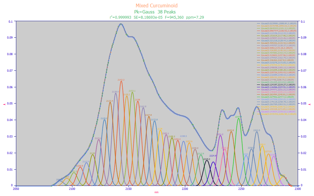
Fig. 5 Constant-width multiple Gaussian fits to FTNIR wavelength spectra for for mixed curcuminoid standard, 2050-2300 nm

The mixed standard's addition of DMC and BDMC does produce a dramatically different spectra (Fig. 5) with a good deal of 2230-2300 nm absorbance that is not seen with pure curcumin. Here we see almost the same shared Gaussian a₂ width, 3.18, 38 peaks, and a respectable fit. Note the large measure of spectral information from 2200 nm upward arising from the other curcuminoids. It is why this band is seen as so attractive for individual component curcuminoid modeling.

FTNIR Spectroscopy of Turmeric - 2100-2300 nm WL Band

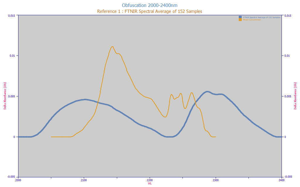
Fig. 6 FTNIR average spectra from 152 turmeric samples, 2000-2400 nm

The news is less good when we view the averaged turmeric spectra in this wavelength band. There is a good deal of 2000-2100 nm absorbance not seen in the curcuminoid samples. There is also a considerable measure of 2300-2400 nm absorbance in the turmeric samples not seen in the curcuminoid powders. We were unable to peak fit this spectra to the same ~3.25nm widths seen in the curcumin or mixed curcuminoid fits (PeakLab has an upper limit of 50 peaks). In Fig. 6, the baseline was anchored at 2230 nm as well as the two boundaries.

The benefits seen in terms of the separation of component spectral signatures in the 2100-2300 nm band are certainly diminished by additional absorbances in the turmeric that are very strong at the two bounds of the curcuminoid band. One would have to believe that these obfuscating absorbances from non-curcuminoids are likely to penetrate well into the modeling band from each side.

Powder vs. Liquid Spectra - Particle Size

We expect this NIR modeling to be much more challenging than the UV-VIS of Part I. Part of our reasoning is the aforementioned obfuscating absorbances in the modeling bands. Turmeric, a natural agricultural product, is known to contain a very large number of components (some authors have reported up to two hundred) and its curcuminoid content and fractions can vary immensely from one sample to the next. The additional absorbances of non-curcuminoids in the modeling bands are thus not surprising. The average curcuminoid content is about 4% of the overall solids in a turmeric powder. On average, 96% of the turmeric is non-curcuminoid.

These other non-curcuminoid components are likely present, to at least some measure, in the solvent extracts of the turmeric used in this UV-VIS spectra white paper. In that case, however, the chromatography gave a clean curcuminoid signature from about 300 nm upward, and in the UV-VIS direct spectral models we realized a superb rČ of 0.994 despite a weaker S/N (3.5 significant digits at the noise floor). Here we have the higher FTNIR resolution and a stronger S/N (4.7 significant digits at the noise floor).

The chromatography was adjusted here, as in the UV-VIS Part I of this white paper, for dry solids so moisture differences in the powders were not a factor in the chromatographic reference values. What could not be accommodated was the intrinsic issue of the particle size densities of the turmeric powders.

You may wish to refer you to an excellent Applied Optics paper, "Quantitative reflectance spectra of solid powders as a function of particle size". Although this paper does not specifically reference turmeric powders, if you look closely at Fig. 10 in this reference, you will see wavenumbers comparable to this FTNIR data (4300-6060 cm^-1). In the UV-VIS of Part I, we could track the amplitude of the spectra with the magnitude of the total curcuminoids. That is not the case for these powder NIR spectra. We believe this is because the amount of curcuminoid, the amount of obfuscating non-curcuminoid, and the particle size of the powder, are all impacting the reflectance measured in the spectra.

We begin with these important pieces of information. In both NIR modeling bands, we have non-curcuminoid spectral information that will impact the absorbances. We also know that even with basic sieving to remove the larger or aggregated particles, there can be significant differences in spectral magnitudes of samples that appear virtually identical in the chromatography. Two turmeric samples with with essentially identical curcuminoid chromatography can have very different spectra as a consequence of the optics of powder reflectance as well as non-curcuminoid content.

It is a great deal for a modeling algorithm to sort. It is why PLS (partial least squares) is seen as so useful to chemometric modeling since its indirection in constructing latent factors could ideally isolate wavelengths where the principal curcuminoids can be estimated and also latent variables associated with the particle distribution density, all of which will impact the reflectance measured in the spectra. In fairness, no linear system such as PLS, or an eigendecomposition system, such as PCR, is going to generate what would be seen in a modeling that included, for example, the moments from a laboratory particle size analysis. We don't expect to see non-linear effects modeled with full permutation direct spectral modeling either, but we can hope to create linear models that are of a sufficient prediction accuracy.

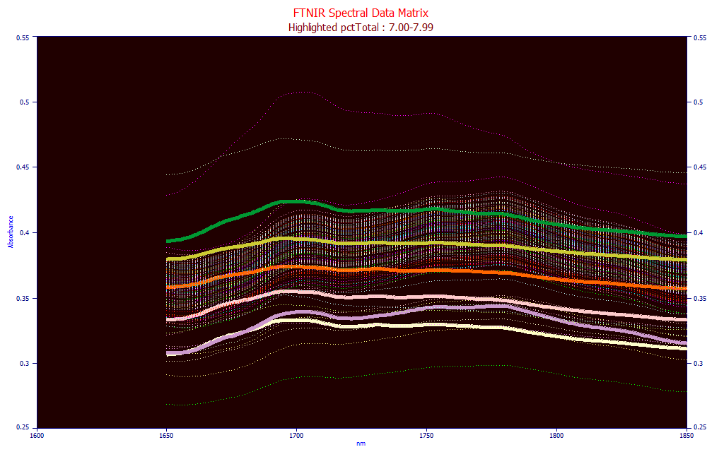
Fig. 7 FTNIR Powder Spectra with total curcuminoids 2.60-2.69 highlighted

In the Fig. 7 plot, we see all of the spectra in the modeling matrix which have a total curcuminoid value between 7.00-7.99 (the samples plotted vary from near zero curcuminoid content up to about 14%). It is fair to say the amplitudes of the spectra are not proportional to total curcuminoids.

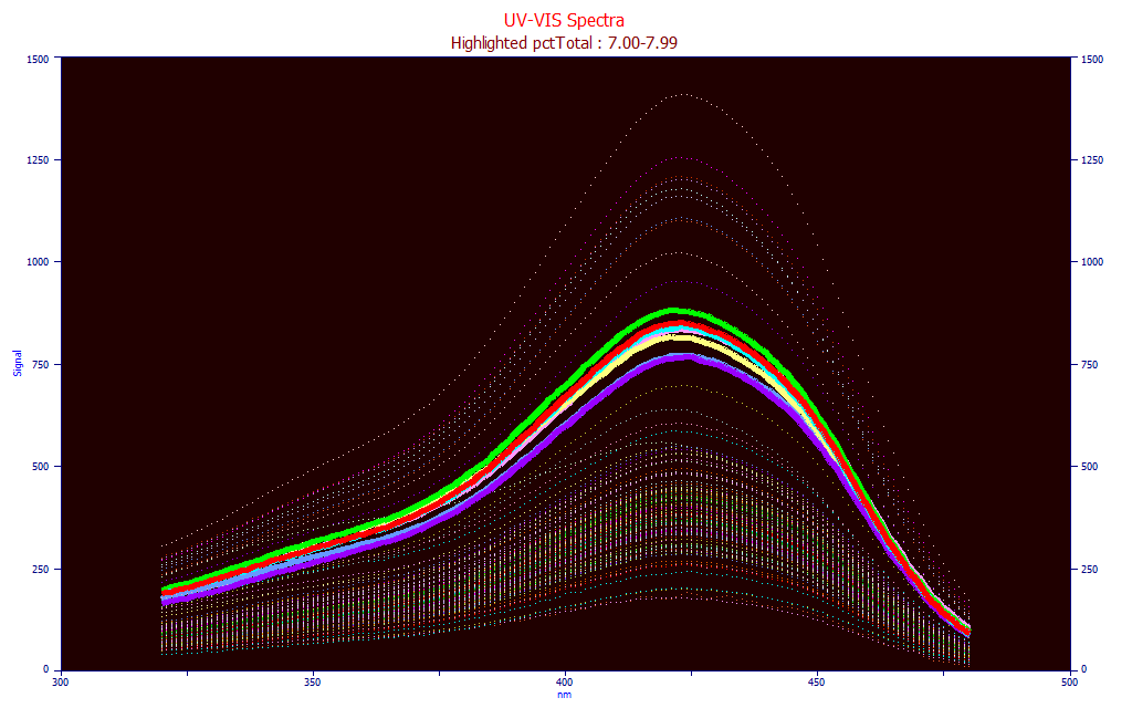
Fig. 8 UV-VIS Liquid Spectra with total curcuminoids 7.00-7.99 highlighted

In the Part I UV-VIS modeling, we did not show this type of comparison, but we do so in Fig. 8. The same 7-8% total curcuminoid samples are highlighted in the UV-VIS liquid spectra. The magnitudes accurately track the total curcuminoid levels.

Powder vs. Liquid Spectra - Compaction and Relative Humidity

Particle size is more than a primary size and density. There is also the issue of weakly bonded agglomerates as well as strongly bonded aggregates. Powders, when in equilibrium with the moisture in the air, will behave differently as a consequence of relative humidity. This adds one further complication to powder reflectance spectral modeling.

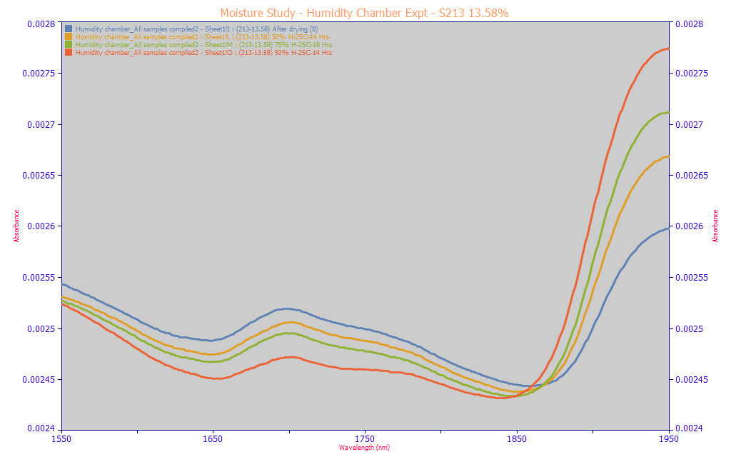
These spectra are from the handheld NIR device described in the Modeling Spectra - Part III - Field Site NIR Data. All are from the same turmeric sample, one with a very high 14% total curcuminoid content. The four spectra above are area normalized 1550-1950 nm spectra of equilibrated powder at 0, 50, 75, and 92% relative humidity. On a weight basis, the powders vary from 11.87% (red - 92% RH) to 13.13% (green - 75% RH) to 13.58% (amber - 50% RH) to 14.63% (blue - 0% RH). This normalization represents a true weight basis picture of this same powder at four different moisture levels.

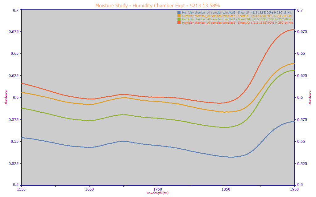
Unlike liquid spectra which is done on a weight basis, powder spectra are done on a volume basis, and the compaction of the powers and the aggregation and agglomeration of the powder particles due to moisture will factor into the spectra. The above plot contains the raw spectra (no normalization). The dry state (blue) has the lowest absorbance in the 1650-1750 curcuminoid band despite having the highest concentration of curcuminoids on a weight basis. The highest moisture state (red) has the highest absorbance despite having an appreciably lower curcuminoid content on a weight basis. Further the 75% RH (green) and 50% RH (amber) samples are reversed from the inverse trend suggested by the blue and red extremes.

You may also wish to refer to the following paper, "Effect of particle size in aggregated and agglomerated ceramic powders". Although this paper specifically references ceramic particles, it does give a sound presentation as to why we might see the spectra effects shown above.

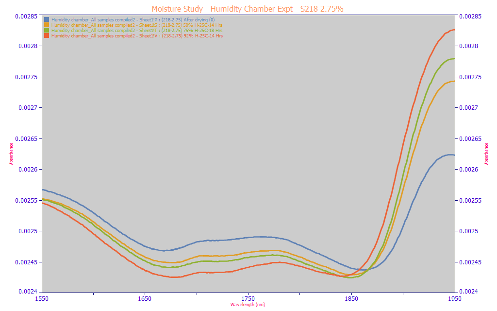
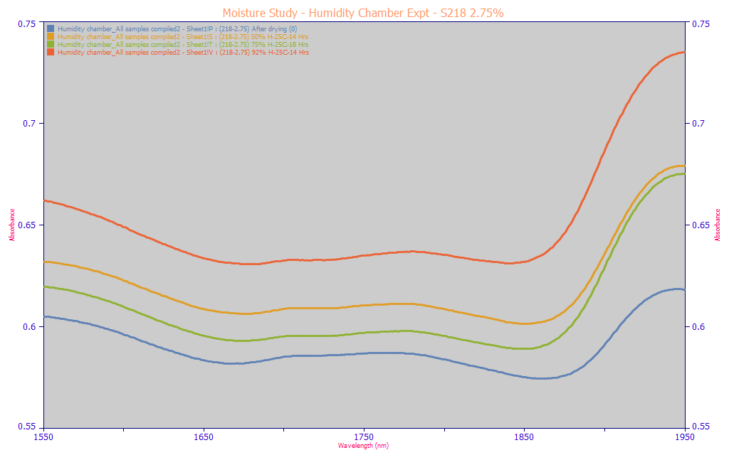
This effect is not an anomaly specific to the very high curcuminoid content in the turmeric powder. The above area-normalized and non-normalized spectra are from a different sample with a much lower 2.75% total curcuminoids. We see the same trends in each. We will also note that this spectrometer uses a custom-built mechanical compaction which seeks to have each powder compacted as identically as possible. This observation is important, for we see for the same powder, a nonlinear effect with respect to ambient moisture. Multivariate linear models can accommodate non-linear effects, but it is a clumsy affair. In spectral modeling, this kind of phenomenon can result in tiny incremental improvements in predictive modeling errors out to unrealistic counts of predictors, factors, or principal components. Further, the efficacy of modeling such nonlinear effects would have to be assumed poor.

Direct Spectral Fit of Total Curcuminoids

At this point, we have a very good sense for the scope of the modeling problem. Some count of predictors will be needed to adjust for particle size of the powders, and some number may be needed to remove non-curcuminoid signal in the modeling bands. Further, if we model the raw spectra, we expect to see major differences in the spectral magnitudes as a consequence of ambient humidity in the test environment, one not easily modeled by a linear relationship with moisture.

Our data matrix for this modeling consists of 146 specific turmeric samples. Each FTNIR spectrum is an average of five separate FTNIR measurements. The total curcuminoid and component values are identical to the values used in the UV-VIS modeling in Part I, an average of three chromatography replicates. Also, as in the UV-VIS modeling, the Y-values consist of dry-solids adjusted values of the total curcuminoids from the chromatography, and as such moisture differences in the turmeric powders have been removed from the Y-values in the modeling.

Using the 2 nm spacing, we will perform a default direct spectral fit to this data. Since we are using a high count of predictors, we will use the default filters to speed up the fitting of the higher predictor count models. A filter works to remove predictors unlikely to appear in the models. If a given wavelength could not make an appearance in the best 5-predictor models, for example, that predictor may be removed from all 6-predictor and higher fits. In this 1650-1850 nm modeling, using 2 nm sampling intervals, the estimated fitting time decreases from 1.5 days to 29 seconds as a consequence of utilizing these filters. An alternative which would fit all possible permutations through eight predictors, omitting all filtering, is possible with a 5 nm spacing, an estimated 1.2 minutes for the fitting. We will begin with the 2 nm spacing since we are hoping to see a benefit from the FTNIR's higher resolution.

Note that the intelligent stepwise fits do not use these full permutation filters, so even if a WL is omitted from the permutation matrix by a filter, it may still appear within one of PeakLab's stepwise models. These are not the simple forward stepwise models you may have fitted in statistics software. Each of these "stepwise" models contains a kind of multidimensional search that seeks to find the best models from a given full permutation model starting point. In this different form of algorithm, a WL predictor that is removed from a model can be added back further along in the process. In general, you will see some benefit in these stepwise models that arise from starting with very effective full permutation models. These allow models up to 15 predictors to be fit.

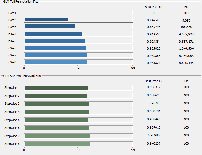
Fig 9. The rČ progression in the fitting, each bar represents an average of the 10 best models of that predictor count

Unlike the UV-VIS modeling, there is no predictive power whatsoever with just a single predictor. The predictions begin only with 2 predictors and are still slightly improving with 8 predictors. The best fits, by the 'leave one out' prediction metric, are the stepwise models which begin with the 7 and 8 predictor full permutation WLs. The best overall prediction goodness of fit rČ is only going to be about 0.94 as contrasted with the greater than 0.99 observed in the UV-VIS modeling of the same turmeric samples.

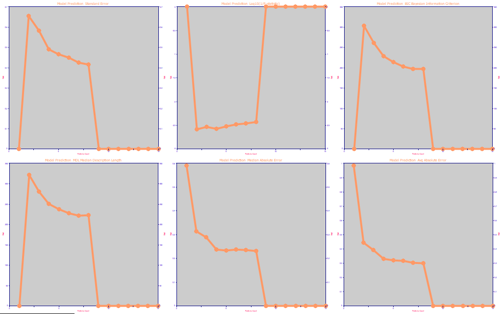
Fig. 10 The prediction statistics as a function of predictor count

Here we chose to look at the ten best models at each predictor count to somewhat smooth the optimization curves. In so doing, the stepwise and sparse PLS models drop out (the models are too few to generate an average of ten), and we are only looking at the full permutation GLM fits. As we described the use of these metrics in the UV-VIS part I fitting, the prediction standard error, median error, and average errors favor the 8-predictor models. The F-statistic selects just 2, the BIC selects 7, and the MDL likewise selects 7.

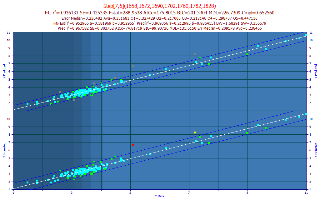
Fig. 11A The selected model plot for the predictive FTNIR model of total curcuminoids

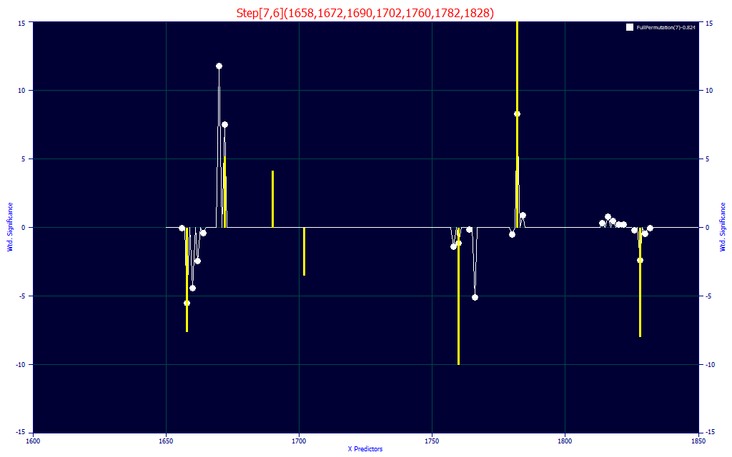
Fig. 11B The selected model and 7-predictor significance plot for the predictive FTNIR model of total curcuminoids

The best model in the fitting, by r² of prediction error, using the leave one out estimate of prediction error, is a 7-predictor model with a r² of prediction of 0.9412. For our purposes, we selected a 7-predictor model (as suggested by the BIC and MDL information criterion), and we sorted the models by compliance with the average of the significance at the different wavelengths. We thus selected a 7-predictor model (Fig. 11A) with an rČ of 0.9361 and an average prediction error of 0.3017 % total curcuminoid. This error is almost three times higher than the 0.113% average error realized from the selected UV-VIS model in Part I.

If we import the model data as separate prediction data, and remove the 6 samples outside a 95% prediction interval of the Y-known vs. Y-predicted fit, the rČ for the model fit (the 'estimation' or 'calibration') improves from .955 to .968. This is shown in the upper portion of the model plot. Whether or not these samples are actually outliers in either the chromatography or spectroscopy, we do have a good overall modeling of the total curcuminoids. There may be significant practical advantages in direct spectral measurement of the powders, and this level of prediction error may be acceptable.

Because of the massive differences between the curcuminoid spectra and the turmeric spectra, we are especially interested in the significance plot (Fig. 11B). The yellow bars represent the selected model, and the white curve is the average of the 100 best 7-predictor models. We note that the 1760 nm has a strong negative correlation, as would be expected from removing non-curcuminoid, and we see the same at 1828 nm. We have a 1782 nm significance that is positively correlated, and this fits with the 1786 nm peak in Fig 1. We do see the one item we are absolutely certain we want to see. The curcuminoid wavelengths in Fig. 1 are positively correlated with the total curcuminoids.

Conventional PLS Modeling of the FTNIR Data and Sparse-PLS models

As with the UV-VIS modeling, we will compare this seven predictor direct spectral fit with the optimal PLS (partial least squares) model. The optimum prediction rČ in a leave-one-out estimation of prediction error occurred with a 7-factor PLS NIPALS model (Systat). This PLS 7-factor model had a prediction rČ of 0.928. The direct spectral fit model above, with a leave-one-out prediction rČ of 0.936, offers slightly more accurate predictions, at least via this leave-one-out prediction metric. The PLS standard error of prediction is 0.451 as compared to this direct spectral fit's standard error of prediction of 0.425.

For Unscrambler, the best 1 nm PLS model, 201 wavelengths, also optimized to 7-factors and a similar leave one out rČ of prediction of 0.092939. The best PCR predictive model used 8 principal components and had a leave one out rČ of prediction of 0.092805. Just as we observed with the UV-VIS modeling, direct spectral fits outperformed PLS and PCR models, and with far fewer coefficients. The selected direct spectal fit model above consists of 8 parameters, as compared to 202 for the Unscrambler PLS and PCR models.

The PLS algorithm works by an iterative set of factor (synthetic variable) extractions that use linear correlations between the dependent variable and every WL specified in the modeling. We have seen references to PLS algorithms that suggest a proficiency at 'latent variable' extraction. In this powder spectra example, that would perhaps imply that the PLS technique will generate hidden variables that essentially map to particle size or to the non-target content that may also be present in the modeling band. With respect to what is or is not possible with linear correlations, we will only note that this kind of unscrambling occurs equally with direct full-permutation GLM spectral fits. In fact, the better direct spectral fits will do this even more effectively, as seen in this example.

We have never encountered spectral data modeling where the optimum PLS was able to match the performance of the best direct full permutation spectral fits. It is reasonably well understood in the prediction science that modeling derived information is often less effective, and may even be dangerous. The relationships that map the raw data to a derived factor may not be stable, and one or more of those can break down and in a black-box system, you may never know. In the financial modeling world, there is a software product that offers over 1000 indicators, all producing derived entities from price or volume time-series data, and there are specialists in the field that refuse to build prediction models using any of them, relying only and entirely on direct price and volume data.

We suspect there was never an issue with PLS fits being seen as some sort of optimum, at least not amongst skilled statisticians who could, with a measure of manual and interactive effort, produce stepwise regression models with a superior prediction to PLS models. PLS was an expedient and convenient alternative to what would otherwise be either a computationally costly full permutation direct spectral modeling, or a tedious manual effort requiring a high level of statistical art.

Although we assert that an automated, intelligent, direct spectral modeling, is much superior to stepwise regression and produces better predictive models than PLS, we also introduce a 'PLS-like' set of direct spectral models.

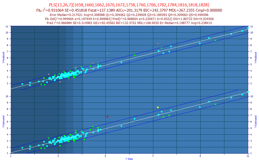
Fig 12. The best sparse-PLS predictive FTNIR model of total curcuminoids with a 2 nm predictor spacing

PeakLab does not offer the conventional PLS algorithm. From our perspective, too much inferential information is dragged into the models. We have seen PLS models whose correlation-based factor extraction gave reasonly little weight to the spectral WLs of the target components, and generated models that were significantly based on the content of non-target materials that happened to be inversely related to the species being modeled, or which even included a high measure of water band information when the material being estimated, due to its hydrophobicity, resulted in lower overall moisture levels in the spectra.

To address what may be the desirability of a larger number of component WLs, PeakLab offers "sparse PLS" models. You can think of these models as 'PLS-like' insofar as they will offer a collection of WLs in the modeling band. Those will be sparse, however, in contrast with the PLS algorithm which includes every predictor in the modeling. In the above sparse PLS model, there are 13 WLs (14 parameters), the WLs shown in the first title of the model plot. Those thirteen predictors will be the 13 wavelengths detected as most significant in the 7-predictor full-permutation general linear models. All of the 7-predictor models whose WLs are all included in this larger set of 13 most significant wavelengths are averaged using weighting that is based on the normalized statistical error of the predictions. In the example above, 26 7-predictor models were part of the weighted average that generated this 13-predictor sparse-PLS model.

Whereas the best NIPALS PLS model (7-factor) of this data generates 102 parameters (1 constant and 101 spectral coefficients, one for each WL), producing a model with a leave-one-out predicted rČ of 0.928, this sparse PLS model generates 14 parameters (1 constant, and 13 spectral coefficients) and produces a model with a leave-one-out prediction rČ of 0.931. Admitted, the improvement is small, but this is realized with just 13 estimated predictors, as opposed to 101, and the model consists of the 13 most significant predictors, and further each of the 7-predictor models combining to produce this sparse-PLS model will be statistically significant in every predictor (only models with all predictors statistically significant are retained in the full permutation fitting).

A sparse-PLS [nsig, navg, npred] model is one where the most nsig significant predictors produce an optimal WL set, and it is populated with navg models, each consisting of npred predictors. You can readily equate the npred predictor count with a factor count. As to whether or not the additional predictors offer a more stable prediction, in the real world there is the obvious tradeoff of more WLs to soften an anomaly at any given predictor, but a greater count of predictors where such anomalies might appear. Since those could easily arise from trace contaminants as well as trace amounts of other species that may have been weakly represented or absent in the model data, one could argue that a sparse-PLS model is adding rather than diminishing risk. Still, a sparse-PLS model will offer comparable or better performance than the optimum PLS-model, and it will do so with far fewer predictors, and with each of these assured significant.

Changing the Sampling Width to 5 nm for an Unfiltered Full Permutation Direct Spectral Fitting

An x-spacing of 5 nm allows all permutations through 8-predictors (about 120 million models) to be fit in a little over a minute on a 4-core machine. The best performing model, by predicted average error, was an 8-predictor model.

Fig 13A. The best predictive FTNIR model of total curcuminoids with a 5 nm predictor spacing, all permutations fitted

In what we had hoped to see, the 2 nm spacing did produce a stronger predictive model, even with every possible 5 nm spaced permutation fitted through 8 predictors. The best 2 nm spaced filtered fit had an rČ of prediction of 0.9412 as compared to 0.9358, with the full permutation of 5 nm spaced fits. The FTIR's resolution is as good as the peak fitting in Fig. 1 indicated.

For this 5 nm spaced data, the conventional NIPALS PLS fit (Systat) optimized to 7 factors. It was also weaker with the 5 nm spacing, although the difference was very small. The 5 nm spaced fit produced an rČ=0.9276 PLS leave-one-out prediction, compared to 0.9282 with the 2 nm spaced data.

To see if fitting every possible permutation of 2 nm spaced models (no filter) produced an even better fit, we would be looking at about 1.5 days for the fitting, with a very good chance of seeing no benefit for all of the trouble. Instead we will use an option to refit the models saved for evaluation to a unit column density (1 nm in the case of our data). We would never under any circumstance fit a 1 nm spacing in this data by brute force - the estimated modeling time would require 1.1 years and fit 60 trillion permutations!

Implementing a 1 nm Refinement on the Full Permutation 5 nm Fits

In this refinement, we use the 5 nm spaced data, we see the same 120 million full permutation models fitted, but the 8000 models retained for evaluating predictions see additional fitting. The fitting time little changed, still a little over 1 minute. In this algorithm, additional models are fitted for each of the 5 nm-spaced wavelengths shifted 1 nm and 2 nm down, and 1 nm and 2 nm up, to see if this 1 nm resolution of that predictor adds any modeling benefit.

Fig 13B. The best predictive FTNIR model of total curcuminoids with a 5 nm predictor spacing, all permutations fitted, with 1 nm refinement

The best model for average prediction error is now a 9-predictor stepwise model. The 5 nm spaced fit has improved from rČ=0.9358 (average prediction error=0.3015) to rČ=0.9451 (average prediction error=0.2850). This is slightly better than the rČ=0.9412 (average prediction error=0.2954) for the best 2 nm spaced fit using the prediction filters. This 1 nm resolution fit is one of those that would have been fitted were we to do a 1 nm full permutation fit. For a 1-9 predictor full permutation matrix with a 1nm spacing, we would be looking at a human lifetime on current computers.

Strategies to Reduce Prediction Error in Specific Quintiles

While there is likely little to nothing to be gained by any form of brute force fitting requiring more than say a minute or so, we will mention modeling strategies that can sometimes reduce prediction error in certain bands of the data.

The five distinct colors in the background of the model plots correspond with the 5 quintiles in the Y-variable, here the total curcuminoids from the chromatography. If the dynamic range of the modeled variable is too great, you may not like the predicted average absolute errors in one or more of the quintiles (shown in the third title line in the model plots). You may be able to weight the data so that the prediction accuracy favors the largest or smallest quintile. PeakLab offers a built-in weighting where each sample is weighted by 1/Y^p. A typical value of p is 1.2-1.3.

You can also create a branch model where you select the a different model for each quintile, the specific model that offers the best prediction in that quintile. You would use the overall model, ie. Fig 13B, to determine which of the five separate quintile models to use for the final prediction. You may be able to gain up to a 10% improvement in prediction accuracy in each quintile by branching to the model that furnishes the optimum predictions for a given quintile.

You may also, if your sample size permits, fit the higher and lower Y-value data to separate models. This approach may offer significant prediction improvements if the optimum wavelengths vary with the amount of the variable that is being estimated. We have observed exactly this in our turmeric powder FTNIR spectral modeling.

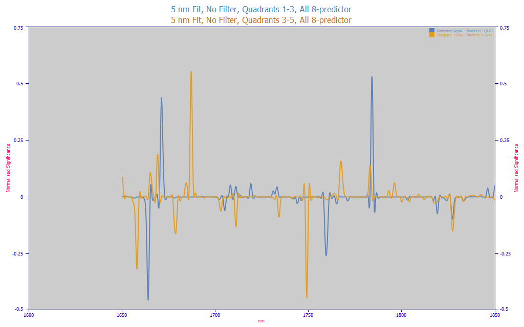
Fig 13C. Comparing the significance WL map for 5 nm predictor spacing, 1nm refinement, all permutations fitted, Quintiles 1-3 vs Quintiles 3-5

The blue curve is the significant wavelength map for the retained 8-predictor models when fitting 5-nm spaced data, no filters, 1 nm refinement, to just the turmeric spectra whose known total curcuminoids are in quintiles 1-3. The amber curve is significant wavelength map for the retained 8-predictor models when fitting the data in quintiles 3-5. Although we could endlessly speculate, we do not know why the higher curcuminoid samples have a different spectral map than the lower curcuminoid samples.

If you see this effect, a high concentration and low concentration model may make a great deal of sense. The errors in all quintiles may be improved. With respect to having a sufficiency of data for this kind of partitioning, experienced statisticians conservatively suggest never fitting fewer data sets than 10 * count of predictors. While that is not always possible, you may wish to keep this guideline in mind when partitioning models or when fitting spectral data matrices in general.

Fitting the Total Curcuminoids to the 2100-2400 nm Band

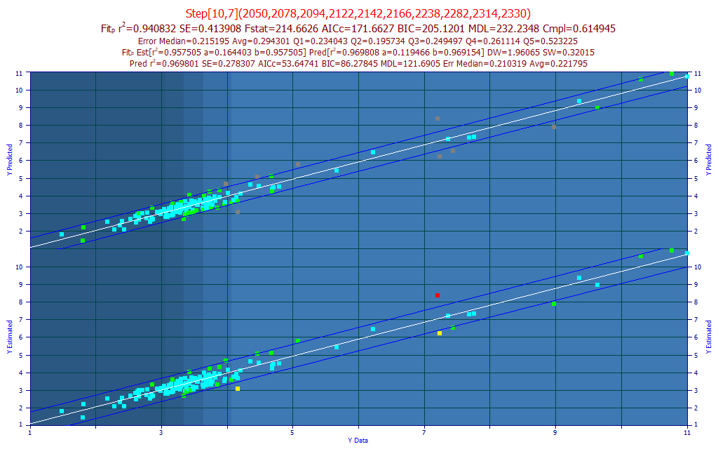
Fig 14. The best predictive FTNIR model of total curcuminoids in the 2100-2400 nm band

Based on the obfuscation shown in Fig. 6, we were not optimistic. There was too much occluding information sullying the spectra of the curcuminoids in this band. With two discrete regions of spectra, we tried fitting 2050-2225 nm and 2225-2400 nm, but both attempts were inferior. In the model plot above, we fit 2050-2400 at a 4 nm spacing, and realized a fit reasonably close to the 1650-1850 nm fit. In this case, the best model was a smart stepwise fit with 10 predictors that began with one of the 7-predictor full permutation GLM fits.

The optimized NIPALS PLS fit (Systat), 2 nm spacing, 101 wavelengths, 9 factors, produced a 0.9274 rČ of prediction.

Although the separation between the three curcuminoid components was especially good in this higher WL band, the additional absorbances from other non-target compounds in the turmeric limited what was possible in the modeling. Although it was impressive that this 10-predictor model was able to unscramble the curcuminoids from the non-curcuminoids in this band as well as the 7-predictor model in the 1650-1850 band, our preference would be for the simpler of the two models, the one in the 1650-1850 nm band.

Direct Spectral Fit of BDMC (bis-demthoxycurcumin)

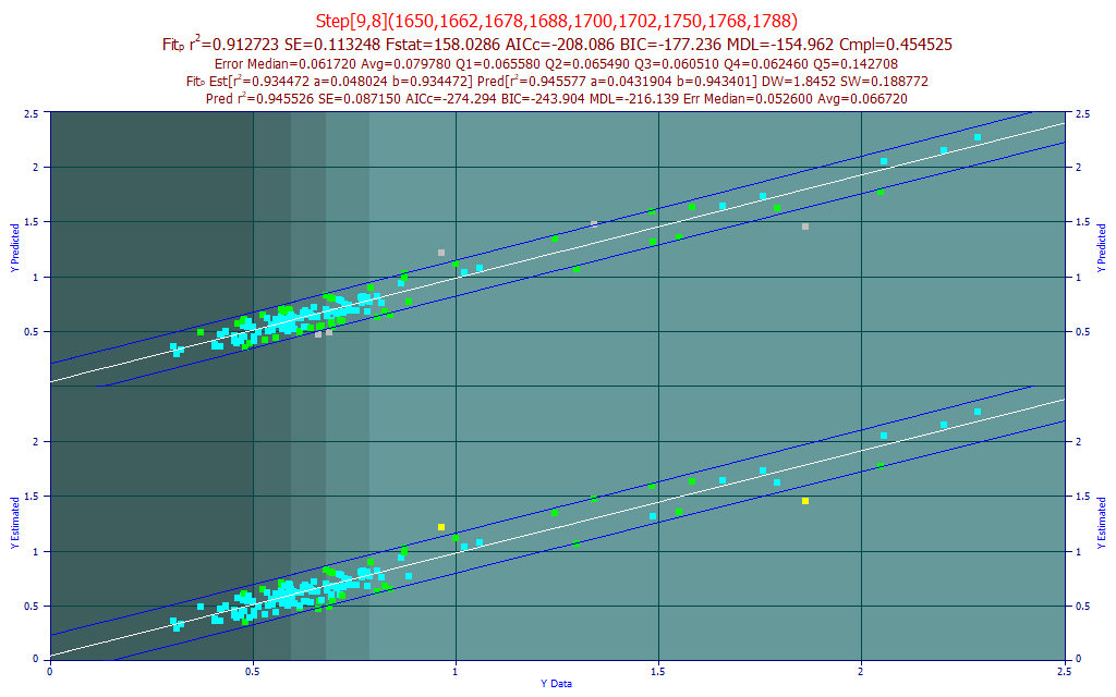
Fig 15. The best predictive FTNIR model of BMDC in the 1650-1850 nm band

Using the same procedures as above with the BDMC component data, we have a weaker fit, an average error of .08% BDMC in turmeric samples that vary from 0.3-2.5% BDMC. The best predictive model was a 9-predictor stepwise model where one additional predictor was added to an 8-predictor GLM fit.

The best Systat PLS model was 9-factor, with a leave-one-out predicted rČ of 0.8815.

For Unscrambler, the best 1 nm PLS model, 201 wavelengths, also optimized to 9-factors and a similar leave one out rČ of prediction of 0.8837. The best PCR predictive model used 7 principal components and had a leave one out rČ of prediction of 0.8606. Again, the best direct spectral fits outperform PLS and PCR models. Here the selected direct spectral fit has 11 parameters, again compared to 202 for the Unscrambler PLS and PCR models.

Direct Spectral Fit of Curcumin

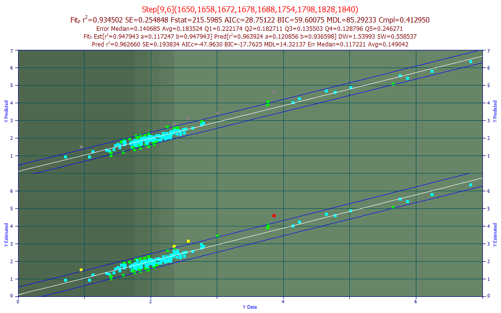
Fig 16. The best predictive FTNIR model of curcumin in the 1650-1850 nm band

The best direct spectral fit to the curcumin component was also a 9-predictor stepwise model, this built upon 6-predictor GLM model starting point. The prediction rČ of 0.934 makes this fit reasonably close in prediction accuracy to that of the total curcuminoids.

The best Systat PLS model was 9-factor, with a leave-one-out predicted rČ of 0.9101.

For Unscrambler, the best 1 nm PLS model, 201 wavelengths, also optimized to 9-factors and a similar leave one out rČ of prediction of 0.9080. The best PCR predictive model used 8 principal components and had a leave one out rČ of prediction of 0.8833. Once more, the best direct spectral fits outperform PLS and PCR models.

Direct Spectral Fit of DMC (demethoxycurcumin)

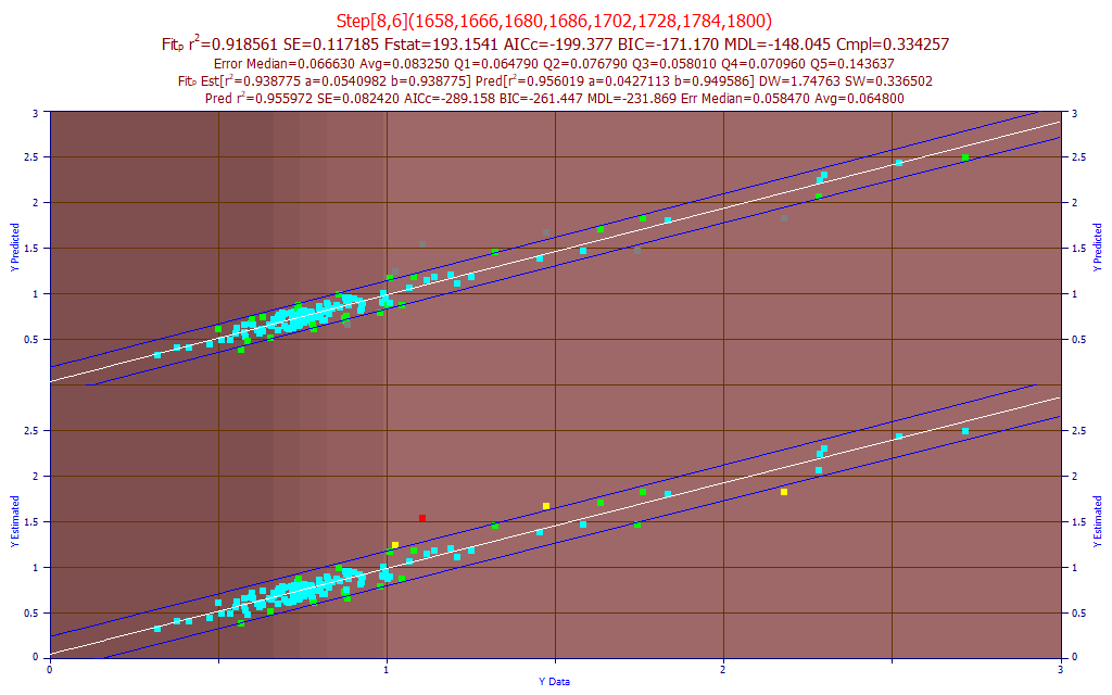
Fig 17. The best predictive FTNIR model of DMC in the 1650-1850 nm band

The difficulty in fitting the DMC component that we observed in the UV-VIS modeling, is also true in the FTNIR modeling. The best model was an 8-predictor stepwise model with a predicted rČ of .9185. This is a good example of the smart stepwise algorithm compensating the omission of certain WLs from the fitting as a consequence of implementing the filters for a much faster fitting. The top 50 models for prediction were all 6 to 8 predictor stepwise models, fits that were omitted from the filtered permutation fitting.

The best Systat 2 nm PLS model was 7-factor, with a leave-one-out predicted rČ of 0.9036.

For Unscrambler, the best 1 nm PLS model, 201 wavelengths, also optimized to 7-factors and a similar leave one out rČ of prediction of 0.9050. The best PCR predictive model used 7 principal components and had a leave one out rČ of prediction of 0.9026. Yet again, the best direct spectral fits outperform PLS and PCR models. Here the selected direct spectral fit has 9 parameters, again compared to 202 for the Unscrambler PLS and PCR models, and 102 for the Systat PLS.

PCR (Principal Component Regression) Spectral Modeling

PCR (principal component regression) is sometimes used as an alternative to PLS modeling. Instead of extracting factors based on correlations, principal components are extracted in an eigendecomposition and used for the weights in the iterative construction of the model instead of successive linear correlations. Like PLS, the indirect variables are converted to spectral parameters where each wavelength in the modeling band of predictors has its own coefficient. In all of the instances of our testing PCR models against PLS models, we never encountered a case where PCR outperformed PLS for prediction accuracy.

We suspect many users of PCR expect it to separate the target content from non-target spectral content, as in transforming the spectrum in Fig. 2 to the spectrum in Fig. 1.

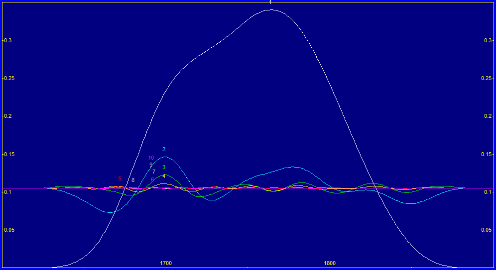
Fig 18. The reconstructed data from an eigendecomposition principal components for the average turmeric spectra in Fig. 3

This is close to an optimal SSA (singular spectrum analysis) eigendecomposition of the overall average turmeric spectrum in Fig. 2. It used the covariance forward-backward algorithm with a covariance matrix order of 40. The first principal component in white lacks the higher resolution of the full data and it looks nothing like Fig. 1, the spectra of mixed curcuminoids. The second principal component, in blue, does have a peak near the primary curcuminoid wavelengths, as do the 3rd (green) and 4th (yellow) principal components. Note that the principal components two and higher plot at the mean of the data for visualization purposes.

We know absorbances begin at 0 and every component is additive, much as in the peak fits in Fig. 1-5. Clearly the second and higher principal components are anharmonic oscillations with both positive and negative swings.

PeakLab does offer eigendecomposition of data matrices. Here we independently fit the reconstructed data from each eigenmode and perform a total curcuminoids fit as was done using the raw data matrix:

The full (original) data is shown in the last line of the table. We were surprised to see a data matrix consisting of the reconstructed data from the second eigenmode (the blue curve above) come quite close to matching the fit to the overall data.

Eigendecomposition or SSA separates based on the power or variance in the signal. Since we have some experience with eigendecomposition (one of the authors of this white paper is the author of AutoSignal), we can share that we see two issues with PCR for spectral modeling. First, eigendecomposition is far more useful for separating oscillations in time-domain waveform signal data. It really cannot deconvolve peak spectra. Two eigenmodes, for example, can exactly capture a full machine precisio single sinusoid. Further, those captured waveforms do not have to be sinusoids. They can be anharmonic.

Although a peak can be viewed as one-half of a waveform cycle oscillation with truncations to zero at the bounds, only the first principal component retains the peak character of the data and all of the other components are oscillatory.

Consider what a separation based on power and variance implies. If there are two overlapping peaks, the first principal component will capture the highest power peak at each frequency. In other words, a given principal component changes peaks as the power of the two overlapping peaks swaps prominence. There can be sharp discontinuities in the first derivative of the reconstructed data from the principal components. The principal component algorithm will also generate edge effects, so you will need to process those eigendecompositions using a wider band than will be used in the modeling.

Principal Component Fitting

PeakLab does have an option where every full permutation fit can specify a maximum count of principal components. This is done directly in the computation of the parameters in the fitting procedure. If you specify a maximum principal component count of 6, all 7-predictor and higher fits will compute parameters using only the first six principal components in the regression matrix. Because this will generally involve millions of fits, the processing time will increase somewhat. It is a useful procedure to avoid the fitting of noise.

Fig 18. The best total curcuminoids fit when a maximum of 6 principal components are permitted in the fitting

The above model plot shows the best fit when specifying a maximum of six principal components in every fitted model. Here the prediction is as strong as the standard (non-principal component) fit we selected in Fig 11A. In this example, an assumption is made that the spectral signal in all eigencomponents seven and higher either have no predictive value, or cannot be trusted to consistently furnish such since the singular values have a very low magnitude.

NIR Spectral Modeling

We hope this white paper has illustrated a useful approach for intelligently building difficult NIR models as well as to demonstrate the merits of direct spectral fits.

Direct spectral fits are simple to compute, easy to understand, have very few coefficients in contrast with PLS and PCR models, and we have found only consistently stronger predictions. Further, the ugly black box aspect of things is gone. It can be disconcerting, for example, to fit the NIPALS PLS model of a given factor size to the same data in several different programs and get three different sets of model coefficients and prediction goodness of fit values. The results from direct spectral fits are easily reproduced using any high-quality statistics package. You can think of full permutation fitting as a methodology more than an algorithm - a fast search procedure for the optimum set of predictors in a simple multivariate model.

We will close with an illustration of the non black-box nature of direct spectral modeling. Here is an excerpt from a model fit from PeakLab:

Rank 1 Step[8,4](1656,1672,1682,1688,1702,1750,1782,1828)

Data: ... - 146 Observations

Fit Statistics

   r²       SE       F-stat       AICc       BIC       MDL       DOF

0.9548032      0.3591034      361.77344      127.61999      155.82642      185.22671       137

Parameter Statistics

 Parm      Value      Std Error      t-value      95%ConfLo      95%ConfHi      P>|t|

Constant      3.239783179      0.650219542      4.982598911      1.954018763      4.525547596      0.00000

   1656      -306.870623      41.07722557      -7.47057814      -388.098011      -225.643235      0.00000

   1672      619.1681358      147.1152543      4.208728313      328.2578401      910.0784314      0.00005

   1682      -812.219338      242.9482872      -3.34317787      -1292.63286      -331.805812      0.00107

   1688      1116.082578      182.6781781      6.109556102      754.8490466      1477.316109      0.00000

   1702      -403.680348      103.9198837      -3.88453426      -609.174770      -198.185927      0.00016

   1750      -590.077783      86.62757091      -6.81166258      -761.377846      -418.777720      0.00000

   1782      547.7031879      61.07093809      8.968311362      426.9396087      668.4667671      0.00000

   1828      -166.914439      26.81370582      -6.22496718      -219.936697      -113.892180      0.00000

This is an excerpt from Systat's GLM output using the same data and set of predictors:

We would expect to see this constancy in every statistics application that implements GLM (general linear model) multivariate least-squares modeling.

Design of a Handheld NIR Spectrometer for Powders

We will now present a final white paper where we develop a handheld device for measuring the curcuminoid levels in commercial turmeric powders: Modeling Spectra - Part III - Field Site NIR Data