PeakLab v2 Documentation Contents R2N Software Home R2N Software Support
Voigt
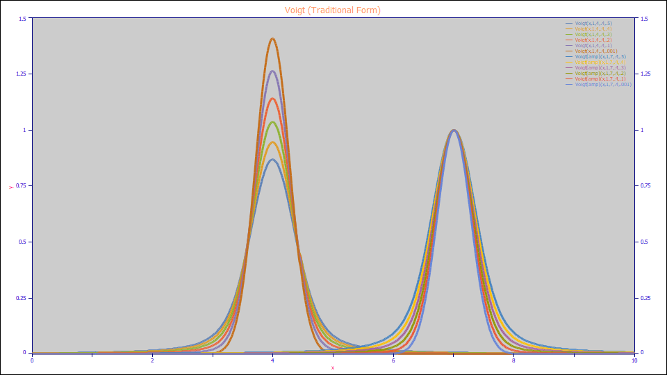
Voigt (Area, Traditional Form)
The traditional Voigt peak with a0 as the peak area is defined as follows:
a0 = Area
a1 = Center (mode)
a2 = proportional to Gaussian Width (Gaussian SD=a2/sqrt(2))
a3 = proportional to Lorentzian/Gaussian Width ratio (Lorentzian width=a2*a3)
Built in model: Voigt
User-defined peaks and view functions: Voigt(x,a0,a1,a2,a3)
Voigt (Amplitude, Traditional)
The traditional Voigt peak with a0 as the peak amplitude is defined as follows:
a0 = Amplitude
a1 = Center (mode)
a2 = proportional to Gaussian Width (Gaussian SD=a2/sqrt(2))
a3 = proportional to Lorentzian/Gaussian Width ratio (Lorentzian width=a2*a3)
Built in model: Voigt[amp]
User-defined peaks and view functions: Voigt[amp](x,a0,a1,a2,a3)
Voigt (Area, Gaussian and Lorentzian Widths)
The Voigt peak fitting the two widths directly with a0 as the peak area is defined as follows:
a0 = Area
a1 = Center (mode)
a2 = Gaussian Width (SD)
a3 = Lorentzian Width
Built in model: VoigtGL
User-defined peaks and view functions: VoigtGL(x,a0,a1,a2,a3)
Voigt (Amplitude, Gaussian and Lorentzian Widths)
The Voigt peak fitting the two widths directly with a0 as the peak amplitude is defined as follows:
a0 = Amplitude
a1 = Center (mode)
a2 = Gaussian Width (SD)
a3 = Lorentzian Width
Built in model: VoigtGL[amp]
User-defined peaks and view functions: VoigtGL[amp](x,a0,a1,a2,a3)
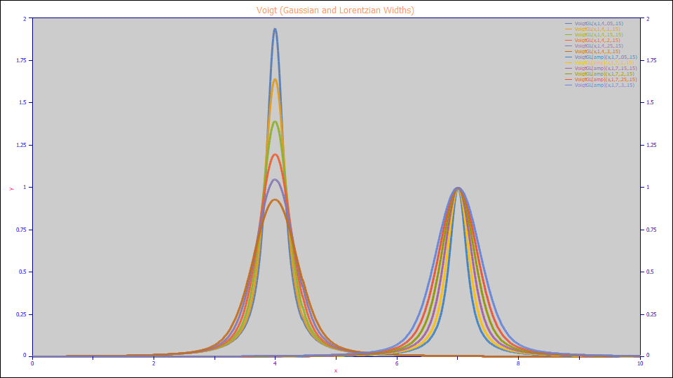
PeakLab offers amplitude and area forms for a Voigt parameterization that directly computes the Gaussian and Lorentzian widths. This enables you to get a standard error and confidence limits for the computation of each of the widths. This is also useful since PeakLab allows you to set the individual a2 and a3 parameters as varying or shared. In the traditional form of the Voigt, sharing a3 means a single ratio of Gaussian to Lorentzian character across all peaks in a spectrum.
Spectral Fitting Considerations
When fitting spectral peaks, the x variable must be proportional to frequency, wave number, or energy. The y variable must be a quantitative measure. As such, you must convert wavelengths to wave number and transmission to absorption prior to fitting.
Depending on the extent of a Voigt�s Lorentzian character, it is not uncommon for some portion of the fitted Voigt's area to lay outside the range of the spectrum being fitted. When this occurs, analytical peak areas will be greater than the measured areas which report a numeric integration using the lower and upper x limits of the data being fitted.
True Non-Linear Deconvolution
Although �deconvolution� seems to be inappropriately applied to all peak fitting, with the Voigt a true deconvolution does occur, and in a manner that no noise is introduced into the analysis. Another way to state the Voigt is Lorentz(a0,a1,a3) � Gauss(1,0,a3). As such, the fitted parameters in the G/L forms directly produce the deconvolved Lorentzian and instrument response function width. Because convolution of an instrument response function is area invariant, one assumes that Lorentz(a0,a1,a3) represents the true peak (as measured by a perfect instrument).
Suggested References
Further information on convolution, deconvolution, the Voigt function, and spectral line broadening can be found in:
(1) Peter A. Jansson, Deconvolution of Images and Spectra, Second Edition, Dover Publications, 2012 (1997,
1984), eISBN-13 978-0-486-29445-2.
(2) https://en.wikipedia.org/wiki/Voigt_profile
Detailed Information about PeakLab's Computation of Voigt Function
The Voigt functions contain complex math since the Gaussian-Lorentzian convolution integrals lack non-complex closed form solutions. PeakLab computes analytic Voigt functions to |e|<1e-10. Although this is a closed form complex model, the complex complementary error function does require an approximating function. There are recent papers that discuss 12, 16, and 20 total coefficient complex error function models and one of these papers reports |e|<1e-6 for a 20 coefficient model.
PeakLab's Voigt function uses a proprietary rational approximation for the complex erfc that was developed using 128 bit floating point rational modeling software and where a model with 26 total coefficients (13 numerator, 13 denominator) was selected. Our development of the analytic Voigt approximation for the original PeakFit software suggested that the errors were so close to analytic precision, we deemed the Voigt function finished. In light of continued publications which address Voigt computation accuracy, the Voigt precision in PeakLab was revisited, and in this section we will share a couple of the evaluations as well as techniques where PeakLab's DSP can be used to evaluate the precision for any external Voigt algorithm.
Comparison with Pure Gaussian and Pure Lorentzian
Rational approximations consist of polynomial terms in both numerator and denominator. Because a polynomial is a sum of terms, there will be the finite double precision floating point limit of 16 orders of magnitude range in any addition. This does mean that a Gaussian with an amplitude of 1.0 which can easily be estimated to the double precision zero limit of 1e-308 in an analytic evaluation of its tails cannot be estimated at such an extreme asymptotic approach to zero using the Voigt with a rational approximation (which will have somewhere in the vicinity of a 1e-16 limit). A pure Lorentzian, decaying by 1/x�, doesn't generally have the compact decay necessary to even approach this finite math addition limit. If there is any Lorentzian character in a spectral peak, any discernible non-zero Lorentzian broadening, the Voigt will easily remain within this bound. We note, however, that the Voigt cannot gracefully simplify to a Gaussian when testing generated Gaussian data with more than this 16 orders of magnitude difference between the peak amplitude value and the values at the bounds. If your peak fits to the Voigt produce the 1e-12 bound on the a3 Lorentzian width, you should assume that no Lorentzian character was detected in the fitting, and you should probably proceed to fit a simple Gaussian. A spectral peak formed by count statistics, for example, is generally fit to a Gaussian.
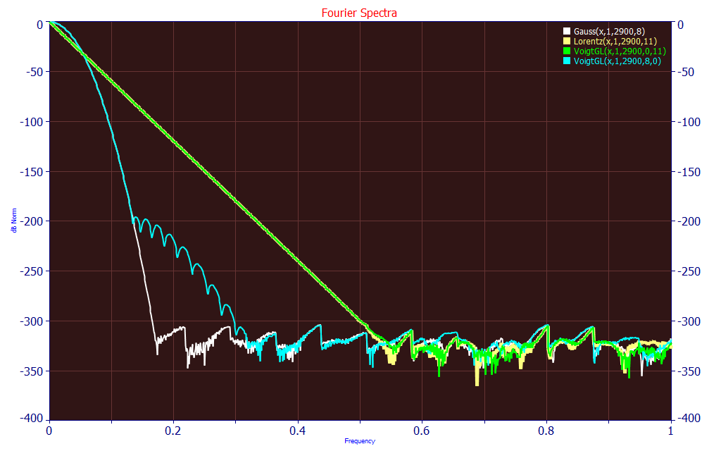
We generated data containing 10,001 values ranging from x=2500 to x=3500 cm-1, and constructed Voigt, Lorentzian, and Gaussian peaks at x=2900 cm-1 as the a1 center, with a Gaussian width of 8 cm-1 and a Lorentzian width of 11 cm-1. The Fourier spectra were generated in the DSP menu's Fourier S/N Estimation option using the csx max rolloff window (with an adjustable alpha = 4.0 for the sidelobe width). This allows all 16 orders of magnitude in the mantissa of double precision data to be visualized in the Fourier domain. The Voigt with the Gaussian zeroed (green) and the pure Lorentzian (yellow) diverge just shy of -300 db, 15 significant digits (-20 db is one order of magnitude). The Voigt with the Lorentzian zeroed (cyan) and the pure Gaussian (white) diverge at about -200 db, 10 significant digits.
Comparison with Mathematica and Maple
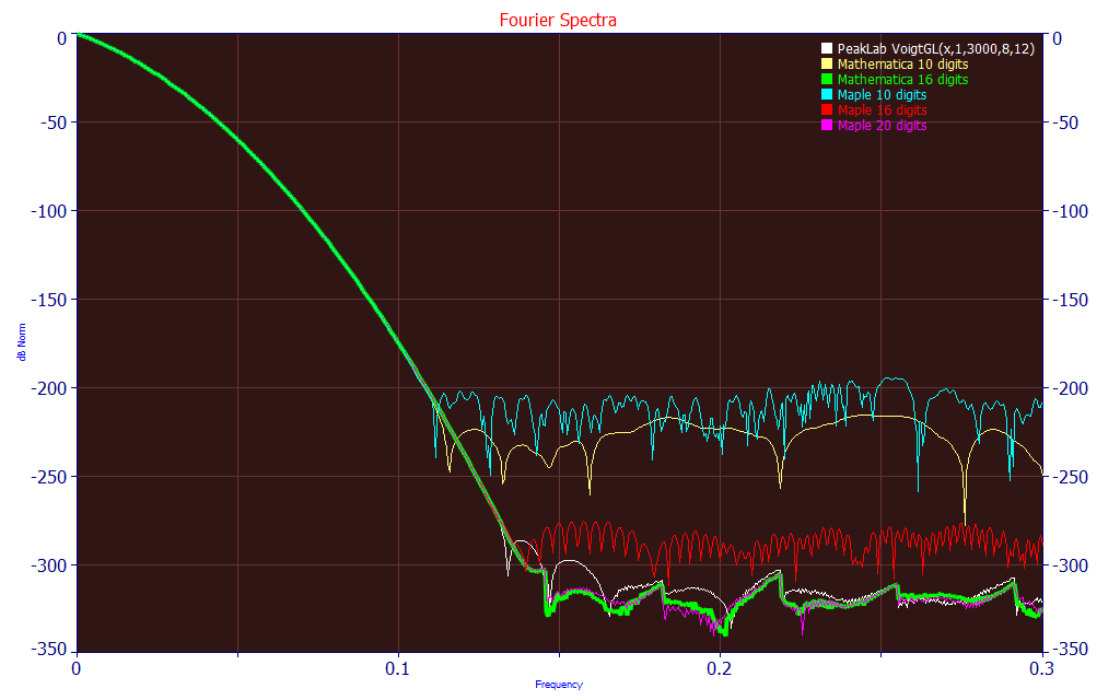
To perform a test with a significant measure of both Gaussian and Lorentzian broadening, we must have an exact reference. For this test, we generated data containing 10,001 values ranging from x=2000 to x=4000 cm-1, constructing Voigt peaks at x=3000 cm-1 as the a1 center, with an a2 Gaussian width of 8 cm-1 and an a3 Lorentzian width of 12 cm-1. The above zoomed Fourier spectra consist of the PeakLab generated VoigtGL(x,1,3000,8,12) in white, the same Voigt data set constructed in Mathematica, one data set with its default 10 digits of precision (yellow) and one with 16 digits (the reference, highlighted, in green). We also have three Maple generated Voigt data sets, one with 10 digits precision specified (cyan), one with 16 digits (red), and one with 20 digits (magenta).
Mathematica: (a0 Re[E^(a3/(Sqrt[2] a2)+(I (-a1+x))/(Sqrt[2] a2))^2 Erfc[a3/(Sqrt[2] a2)+(I (-a1+x))/(Sqrt[2]
a2)]])/(a2 Sqrt[2 \[Pi]])
Maple: (a0*Re(exp((a3/(sqrt(2)*a2)+(I*(-a1+x))/(sqrt(2)*a2))^2)*erfc(a3/(sqrt(2)*a2)+(I*(-a1+x))/(sqrt(2)*a2))))/(a2*sqrt(2*Pi));
We look for where the different sets diverge from the green Mathematica full precision reference. The first set to diverge is the Maple 10 digit precision data, This occurs at about -180 db or 9 significant digits. The next is the Mathematica 10 digit data set at -190 db, about 9.5 digits. The next divergence occurs with the Maple 16 digit data set at about -260 db (13 digits). The PeakLab Voigt follows at about -275 (13.5 digits). The Mathematica 16 digit precision Voigt and the Maple 20 digit precision Voigt diverge at about -305 db (15+ digits). Because the Fourier spectrum uses double precision math, its limit on a normalized decibel plot will be approximately -320 db (16 digits).
Real World Spectral Data
The highest S/N data we have yet seen with real world spectral data was observed with Perkin-Elmer FTNIR data that had 5.3 digits of precision.
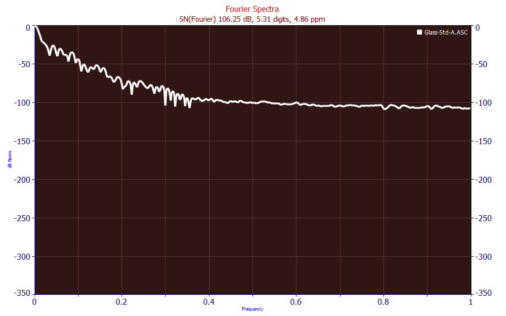
This is a Fourier spectrum of that data set, using the same csx maxRolloff window in the Fourier S/N Estimation option, and db scaled identically to the prior plot. This should give you a sense for the sufficiency of the Voigt model as implemented in PeakLab. The issue with the inability of the Voigt's complex erfc approximation to degrade gracefully to a Gaussian at values that asymptotically approach zero beyond 16 orders of magnitude is purely theoretical since no instrument can generate spectral data that spans that range of numeric values.