PeakLab v1 Documentation Contents            AIST Software Home            AIST Software Support

XPS Baselines

XPS (X-ray Photoelectron Spectroscopy) Baselines

The XPS baselines are available in PeakLab's Baseline option. Unlike Whittaker or BEADS, which rely on smoothness or sparsity, XPS-specific baselines (Shirley and Tougaard) are integral-based. They assume that the baseline at any given point is proportional to the total area of the peaks at higher kinetic energies (or lower binding energies), representing the background of scattered electrons.

The Shirley Baseline

 

The standard Shirley algorithm is often prone to failure if the ROI (Region of Interest) is poorly defined or if it encounters complex doublets. PeakLab utilizes a Multi-Peak Smart ROI variation to address these limitations.

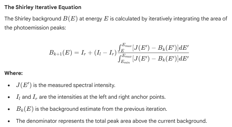
Iterative Area Integration

The baseline is calculated iteratively where the background at a point is proportional to the integrated peak area above that point.

Smart ROI Slicing

To prevent the baseline from "wandering" in noisy data, PeakLab employs an automated slicing mechanism (min_be and max_be) to anchor the baseline to the true noise floor.

Doublet Handling (npeaks)

Standard Shirley can "step" incorrectly between closely spaced peaks. This variation allows for a specific peak-count argument to ensure the integration accurately reflects the background transition across multi-component envelopes.

Shirley Baseline: Multi-Peak Iterative Standard

The Shirley baseline is the rigorous standard for X-ray Photoelectron Spectroscopy (XPS) analysis. It operates on the physical principle that the background at any given energy point is directly proportional to the total cumulative area of the photoemission peaks at higher kinetic energies (lower binding energies).

Why PeakLab Refined the Algorithm

Standard Shirley implementations found in many legacy packages often suffer from "baseline diving" or "stepping" artifacts. These occur because the traditional algorithm assumes a single, simple peak with clearly defined start and end points. PeakLab’s refined Shirley engine addresses these real-world complexities through several key structural modifications:

     Multi-Peak Awareness (The npeaks Parameter): In XPS, signals frequently appear as doublets (e.g., Ag 3d, Pd 3d) or complex overlapping envelopes. A standard Shirley fit might "step up" prematurely between these peaks. PeakLab identifies the top $N$ peaks in the region and ensures the baseline calculation spans the entire multi-peak cluster rather than treating each peak in isolation.

     Smart ROI (Region of Interest) Management: Instead of forcing the user to perfectly "guess" the baseline anchors, the algorithm uses Robust Peak Detection. It automatically searches outward from the outermost identified peaks to find the true local minima (valleys). This prevents the baseline from being anchored on a peak slope, which is a primary cause of non-physical negative peak intensities.

     Gaussian Pre-Smoothing: To prevent the baseline from "jumping" due to stochastic noise at the boundaries, PeakLab applies a configurable Gaussian kernel (smooth_width) during the initial anchor-point detection. This ensures the $yl$ and $yr$ (left and right) intensity values are representative of the actual background floor rather than a single noise spike.

     Automated Slicing: The algorithm handles both High-to-Low (standard XPS) and Low-to-High binding energy data formats automatically. It slices the data based on your specific min_be and max_be constraints, ensuring the iterative integral calculation is only performed on the relevant spectral window.

The Iterative Process

The baseline is calculated using an iterative area-integration method:

1.   Initial Estimate: A flat or linear background is assumed between the anchor points ($yl$ and $yr$).

2.   Area Integration: The area under the peak (relative to the current background) is integrated from high kinetic energy to low kinetic energy.

3.   Refinement: The background at each point is updated based on the ratio of the partial area to the total area.

4.   Convergence: This process repeats until the change in the baseline shape falls below the specified tolerance (tol), usually within 50 iterations.

Practical Guidance

     When to Use: Shirley is the preferred method for metals and semiconductors where the background is primarily composed of inelastically scattered electrons from the primary photoemission event.

     Setting npeaks: For a doublet like Ag 3d, set npeaks=2. This forces the algorithm to encompass both peaks in a single, continuous Shirley step, providing a much more accurate area quantification for the entire transition.

     ROI Limits: If the baseline appears to "cut into" the peaks, try widening your min_be and max_be values to allow the Smart ROI logic to find better "valleys" outside the peak envelope.

Core References

Shirley, D. A. (1972). High-resolution X-ray photoemission spectrum of the valence bands of gold. Physical Review B.

The Tougaard Baseline Variations

The Tougaard baseline is the most physically rigorous method for background subtraction in X-ray Photoelectron Spectroscopy (XPS). Unlike the empirical Shirley method, which assumes a background proportional to the peak area, the Tougaard model accounts for the actual inelastic scattering of electrons as they exit the sample.

Parameters

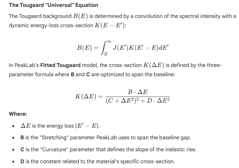
     B Parameter (Intensity or Span): This parameter represents the intensity of the inelastic scattering cross-section. It effectively scales the height of the rising background behind the peak. Adjusted by the optimizer to ensure the baseline connects the left and right ROI anchors.

     C Parameter (Shape or Curvature): This parameter defines the "shape" or curvature of the inelastic tail. It determines how quickly the background rises and levels off as you move away from the peak center. Fitted simultaneously with B to manage the "slope" of the inelastic rise, ensuring the curve "hugs" the data without cutting into peak area.

     D Parameter (Cross Section): Typically held as a constant while B and C are optimized to reach the "tail" region.

Universal Cross-Section

Uses the standard U(E) cross-section but implements an iterative fit to handle the background over arbitrary scan ranges.

Log-Scale DE Optimization (B and C parameters)

Because the Tougaard parameters (B and C) often span multiple orders of magnitude, PeakLab’s Differential Evolution (DE) optimizer operates in log-space. This ensures numerical stability and prevents the genetic algorithm from getting "stuck" in sub-optimal linear regions.

Automatic Parameter Fitting

The algorithm can automatically determine the B parameter (cross-section intensity) by matching the background to the signal levels far from the peak centers.

PeakLab Variations

     Iterative Universal Tougaard: This variation automatically adjusts the baseline height through successive iterations to ensure the background matches the signal level at the low-kinetic-energy side of the spectrum.

     Log-DE Fitting: By optimizing in log-space ($log_{10}(B)$ and $log_{10}(C)$), the genetic algorithm can effectively explore the vast parameter space without becoming biased toward larger values.

     Scan-Range Independence: Our implementation includes an adaptive algorithm that handles arbitrary scan ranges, preventing the "baseline drop-off" often seen in standard Tougaard implementations when the ROI is too narrow.

The "Stretched" Parameter Model

The Tougaard baseline is physically rooted in the inelastic scattering of electrons. However, PeakLab moves beyond the "Universal" constants often cited in textbooks to provide a baseline that actually spans the full breadth of real-world spectral data. In theoretical XPS, the B parameter is often treated as a fixed constant (e.g., 2866 in Ag example below). In practice, using a fixed B often results in a baseline that fails to bridge the gap between the peak and the high-binding-energy background. Instead of a fixed constant, PeakLab treats B as a dynamic "stretching" variable. Our Differential Evolution (DE) optimizer searches for a B-value (often significantly higher than the theoretical "Silver" constant) that allows the curve to perfectly span the distance from the peak tail to the background floor. This "stretches" the theoretical physics model to account for the entirety of the scattered signal, ensuring a stable and repeatable zero-point for quantification.

Core References

Tougaard, S. (1988). Quantitative analysis of the inelastic background in surface electron spectroscopy. Surface and Interface Analysis.

Tougaard, S. (1997). Accuracy of the non-destructive surface nanostructure quantification optimization algorithm. Surface and Interface Analysis.

Comparing the PeakLab Shirley and Tougaard Algorithms
 

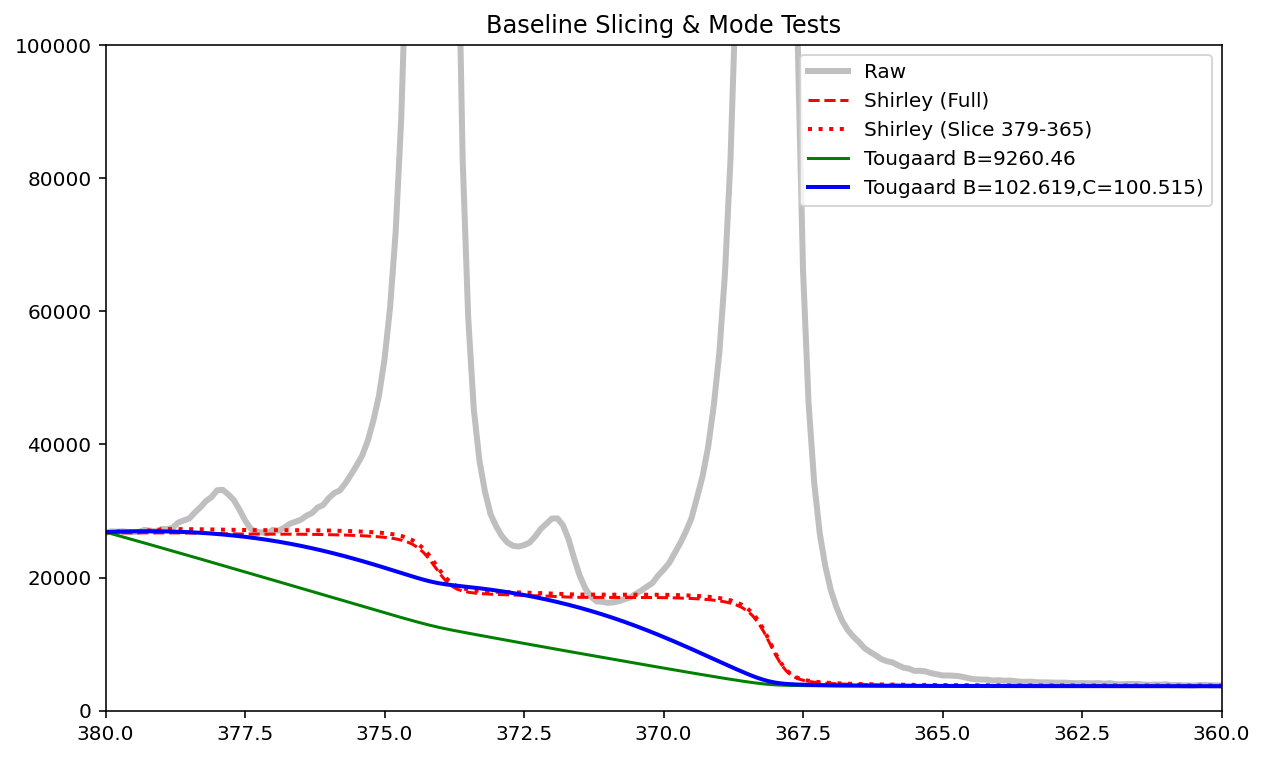
The PeakLab XPS baselines are automated procedures that determine the best parameters to produce a high accuracy quantification for subsequent peak fitting. The above plot shows what what can expect from the Shirley and Tougaard methods.

In PeakLab, the Shirley region of interest is automatically determined as well as the peak count. You should be aware of the Shirley's sensitivity to this ROI and peak count. Two different Shirley computations (two different ROIs) are shown in the red curves. This plot shows the sensitivity to the choice of starting and ending binding energies. The Shirley baseline, while widely used, isn't compatible with the DE optimized Tougaard.

The blue curve is the baseline that PeakLab reports for the Tougaard where B and C are fitted to account the full scatter and to produce a baseline that should offer more accurate quantities for the components. The green curve is the theoretical Tougaard curve inflated to land at the upper binding energy bound.

The PeakLab Quant-First Philosophy

Traditional implementations of Shirley and Tougaard often prioritize theoretical formulas over practical data fitting. PeakLab takes an "Accuracy First" approach, using automated optimization to ensure that every baseline provides a stable, repeatable zero-point for peak area integration.

Tougaard - Beyond the Formula: While the Tougaard universal cross-section is theoretically interesting, it rarely accounts for the full spectrum of secondary electron scatter in real samples. PeakLab uses Differential Evolution (DE) to fit the B and C parameters, ensuring the baseline accounts for the entire scattering background and lands perfectly on the spectral "tail."

Shirley - Context-Aware ROI: A single-peak Shirley is often useless for the doublets and complex envelopes found in modern XPS. Our Smart ROI and npeaks logic forces the algorithm to recognize multi-peak clusters as a single analytical entity, preventing non-physical "steps" between peaks that would otherwise corrupt your quantification.

Automation as a Guardrail: By automating the boundary detection and parameter fitting, PeakLab eliminates the "human-error" factor of manual baseline guessing. This ensures that even if a user is unfamiliar with the underlying physics, the resulting quantification remains mathematically sound and anchored to the physical data floor.