PeakLab v2 Documentation Contents R2N Software Home R2N Software Support
GenHVL
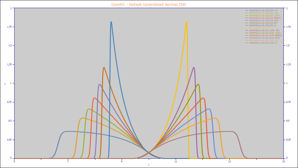
GenHVL - Default Generalized Normal ZDD
By inserting the default Generalized Normal ZDD for the PDF, CDF, and CDFc in the GenHVL template, we produce the GenHVL model:
a0 = Area
a1 = Center (as mean of asymmetric peak)
a2 = Width (SD of underlying Gaussian ZDD)
a3 = HVL Chromatographic distortion ( -1 > a3 > 1 )
a4 = ZDD asymmetry ( -1 > a4 > 1 )
Built in model: GenHVL
User-defined peaks and view functions: GenHVL(x,a0,a1,a2,a3,a4)
Note that the a4 value controlling the skew of the GenHVL peak appears as a3 in the ZDD nomenclature.

GenHVL Considerations
When a4=0, the ZDD becomes a Gaussian and the model reduces to the HVL.
Assuming the instrumental distortions have been removed, in a deconvolution step or in the actual fitting, the GenHVL will successfully model most analytical chromatographic peaks. If you want an analytic peak model with a direct diffusion-type a2 width, as opposed to a kinetic time constant, this may be the only model you will ever need.
This a4 skew adjustment in the ZDD manages the deviations from the Gaussian ideality assumed in the theoretical infinite dilution HVL. This is the statistical asymmetry parameter; small differences in values produce large deviations in shapes. For most IC and non-gradient HPLC peaks, you should expect an a4 between +0.01 and +0.03 (the deviation from non-ideality is a right skewed or tailed).
In most instances, a4 can be assumed constant (shared) across all peaks in the chromatogram. It is strongly recommended that a4 be shared across all peaks and only independently fitted with each peak if the parameter significance allows and you find such necessary. In our experience, across a wide range of concentrations, and across peaks ranging from highly fronted to highly tailed, the fitted a4 was very close to constant.
The addition of this single a4 parameter to an overall fit can result in orders of magnitude improvement in the goodness of fit. The impact of just this one additional parameter in a fit of perhaps many dozens of parameters can be the difference between 5 ppm and 5000 ppm in the unaccounted variance in the fit.
The a4 is also an exacting indicator of the deviation from this ideality. Changes in the a4, in fitting a given standard, may well be indicative of column health. The greater the a4 value, the more the separation is deviating from this Gaussian ZDD assumption of the HVL.
Note that the a4 will be most effectively estimated and fitted when the peaks are skewed with some measure of fronting or tailing. Higher concentrations are very good for this model, assuming that one does not enter into a condition of overload that impacts the quality of the fit.
This model will be least effective in highly dilute samples with a poor S/N ratio since such peaks will generally have much less intrinsic skew.
The GenHVL<irf> composite fits, the model with a convolution integral describing the instrumental distortions, isolate the intrinsic chromatographic distortion from the IRF instrumental distortion only when the data are of a sufficient S/N and quality to realize two independent deconvolutions within the fitting. For very dilute and noisy samples, you will probably have to remove the IRF prior using independent determinations of the IRF parameters.
The GenHVL<ge> model uses the <ge>IRF, consistently the best of the convolution models as it fits both kinetic and probabilistic instrument distortions. Bear in mind, however, that this fit must extract the kinetic instrumental distortion, the probabilistic instrumental distortion, the a4 intrinsic skew to the chromatographic distortion, and the primary a3 chromatographic distortion (very possibly for for each peak). It is recommended the IRF parameters be determined by fits of a clean standard, and the instrumental distortions removed by deconvolving the known IRF prior to fitting more complex peak data.
Since peaks often increase in width with retention time, the a2 will probably be varied (independently fitted) for each peak.
Since peaks often evidence increased tailing with retention time, the a3 will probably be varied (independently fitted) for each peak.
If you are dealing with a small range of time, however, or of you are dealing with overlapping or hidden peaks in a narrow band, a2 and/or a3 can be held constant across the peaks in this band.
If you are addressing gradient peaks, or the overload shapes of preparative chromatography, you will need the Gen2HVL or GenHVL[Y] model where the fourth moment of the peak is also adjusted.
The GenHVL model is part of the unique content in the product covered by its copyright.
Relationship Between the GenHVL Chromatographic Models and the Generalized Normal
The GenHVL, GenHVL[Z], GenHVL[L], GenHVL[Y], GenHVL[T], and GenHVL[V] models use the asymmetric normal generalization in the ZDD and reduce to the generalized normal when there there is no a3 chromatographic distortion and for the [Y], [T], and [V] densities, when other conditions are also met.
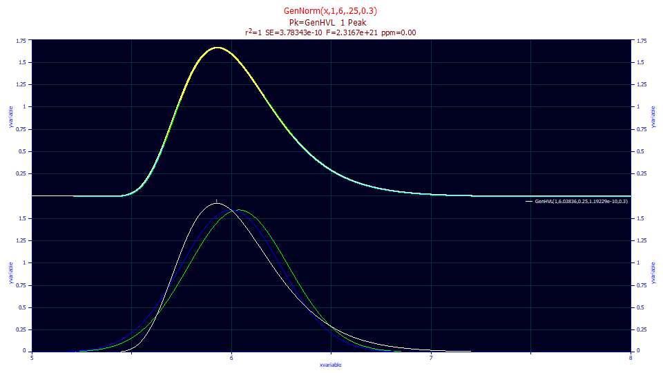
We will generate a standard statistical generalized normal as GenNorm(x,1,6,0.25,0.3):

All of the fits in this study use data essentially free of error.
GenHVL
We now fit the data to the GenHVL model. It uses a generalized normal as its zero distortion density (ZDD) where where a1 is the mean of the asymmetric peak:
"GenNorm(x,1,6,.25,0.3)"
Fitted Parameters
r^2 Coef Det DF Adj r^2 Fit Std Err F-value ppm uVar
1.00000000 1.00000000 3.7834e-10 2.3167e+21 0.00000000
Peak Type a0 a1 a2 a3 a4
1 GenHVL 1.00000000 6.03835655 0.25000000 1.1923e-10 0.30000000
Measured Values
Peak Type Amplitude Center FWHM Asym50 FW Base Asym10
1 GenHVL 1.66921896 5.92827598 0.54929402 1.42364863 1.15470997 1.90368184
Peak Type Area % Area Mean StdDev Skewness Kurtosis
1 GenHVL 0.99997741 100.000000 6.03830768 0.26730627 0.93988068 4.55643791
Analytic Moments
Peak Type FnArea % FnArea FnMean FnStdDev FnSkewness FnKurtosis
1 GenNorm 1.00000000 100.000000 6.03835655 0.26750270 0.94953491 4.64491040
Deconvolved Moments
Peak Type Area Mean StdDev Skewness Kurtosis
1 HVL 0.99922405 6.00066719 0.24894111 0.02443830 2.93924825
Peak Type Area Mean StdDev Skewness Kurtosis
1 Gauss 0.99922405 6.00066719 0.24894111 0.02443830 2.93924825
For the GenHVL, the a3 chromatographic distortion fits asymptotically close to 0.0, as expected. The a2 and a4 exactly match the SD and statistical asymmetry of this generalized normal. The a1's, however, do not match. The fitted GenHVL a1 is the mean or first moment, and not the median used in the GenNorm() generating function. In chromatography, the center of mass is important, and the GenHVL and GenNLC models have been parameterized accordingly.
Also of note is that the integrated higher moments of the GenHVL do not exactly match the analytic moments of the GenNorm[m] ZDD. This is the difference between integrated higher moments of discrete data and an analytic formula for those higher moments, when the skew and/or kurtosis is considerable. The analytic moments will be an exact function of the fitted parameters.
The Deconvolved HVL and Gaussian a1 reflect the fitted underlying Gaussian a1 center, here very close to the 6.0 used in the generating function.
GenHVL[Z]
Next we fit the data to the GenHVL[Z] model which uses the statistical definition of the generalized normal:
"GenNorm(x,1,6,.25,0.3)"
Fitted Parameters
r^2 Coef Det DF Adj r^2 Fit Std Err F-value ppm uVar
1.00000000 1.00000000 2.9529e-10 3.8032e+21 0.00000000
Peak Type a0 a1 a2 a3 a4
1 GenHVL[Z] 1.00000000 6.00000000 0.25000000 4.4673e-10 0.30000000
Measured Values
Peak Type Amplitude Center FWHM Asym50 FW Base Asym10
1 GenHVL[Z] 1.66921896 5.92827598 0.54929401 1.42364863 1.15470997 1.90368184
Peak Type Area % Area Mean StdDev Skewness Kurtosis
1 GenHVL[Z] 0.99997741 100.000000 6.03830768 0.26730627 0.93988068 4.55643790
Analytic Moments
Peak Type FnArea % FnArea FnMean FnStdDev FnSkewness FnKurtosis
1 GenNorm 1.00000000 100.000000 6.03835655 0.26750270 0.94953490 4.64491037
Deconvolved Moments
Peak Type Area Mean StdDev Skewness Kurtosis
1 HVL 0.99922405 6.00066719 0.24894111 0.02443830 2.93924825
Peak Type Area Mean StdDev Skewness Kurtosis
1 Gauss 0.99922405 6.00066719 0.24894111 0.02443830 2.93924825
For the GenHVL[Z], all of the parameters match the generating function as the a3 chromatographic distortion again fits to an effective 0. In the GenHVL[Z] model, a1 is the median of the generalized normal, the mean of the underlying Gaussian.
GenHVL[Y]
The GenHVL[Y] is based on the Generalized Error model. The Generalized Normal [Z] model is a specialization of the Generalized Error [Y] model.
"GenNorm(x,1,6,.25,0.3)"
Fitted Parameters
r^2 Coef Det DF Adj r^2 Fit Std Err F-value ppm uVar
1.00000000 1.00000000 1.4009e-10 1.3518e+22 0.00000000
Peak Type a0 a1 a2 a3 a4 a5
1 GenHVL[Y] 1.00000001 6.00000000 0.25000000 1.2564e-10 2.00000000 0.30000000
Measured Values
Peak Type Amplitude Center FWHM Asym50 FW Base Asym10
1 GenHVL[Y] 1.66921896 5.92827598 0.54929402 1.42364868 1.15470997 1.90368187
Peak Type Area % Area Mean StdDev Skewness Kurtosis
1 GenHVL[Y] 0.99997741 100.000000 6.03830768 0.26730627 0.93988068 4.55643791
Analytic Moments
Peak Type FnArea % FnArea FnMean FnStdDev FnSkewness FnKurtosis
1 GenNorm 1.00000001 100.000000 6.03835655 0.26750270 0.94953490 4.64491040
Deconvolved Moments
Peak Type Area Mean StdDev Skewness Kurtosis
1 HVL 0.99922405 6.00066719 0.24894111 0.02443830 2.93924825
Peak Type Area Mean StdDev Skewness Kurtosis
1 Gauss 0.99922406 6.00066719 0.24894111 0.02443830 2.93924825
For the GenHVL[Y], the a3 chromatographic distortion also fits to an effective 0, and a4 (here the power of the generalized error model) fits to 2.0, the Gaussian decay. As with the [Z] density, which is a specialization of the [Y], all of the standard generalized normal parameters are fitted.
GenHVL[T]
The GenHVL[T] uses this asymmetric normal generalization with the Student's t model. This model asymptotically reduces to the generalized normal [Z].
"GenNorm(x,1,6,.25,0.3"
Fitted Parameters
r^2 Coef Det DF Adj r^2 Fit Std Err F-value ppm uVar
1.00000000 1.00000000 1.3069e-7 1.9417e+16 5.9841e-8
Peak Type a0 a1 a2 a3 a4 a5
1 GenHVL[T] 1.00000014 5.99999857 0.24999952 -1.954e-7 1e+6 0.30000149
Measured Values
Peak Type Amplitude Center FWHM Asym50 FW Base Asym10
1 GenHVL[T] 1.66921899 5.92827573 0.54929396 1.42365103 1.15471014 1.90368417
Peak Type Area % Area Mean StdDev Skewness Kurtosis
1 GenHVL[T] 0.99997755 100.000000 6.03830783 0.26730658 0.93988635 4.55646511
Analytic Moments
Peak Type FnArea % FnArea FnMean FnStdDev FnSkewness FnKurtosis
1 GenNorm 1.00000014 100.000000 6.03835525 0.26750236 0.94954015 4.64492901
Deconvolved Moments
Peak Type Area Mean StdDev Skewness Kurtosis
1 HVL 0.99922420 6.00066708 0.24894063 0.02443549 2.93924839
Peak Type Area Mean StdDev Skewness Kurtosis
1 Gauss 0.99922419 6.00066576 0.24894063 0.02443827 2.93924831
For the GenHVL[T] to become a generalized normal, a3 must be zero and the a4 nu (DOF) parameter must asymptotically approach infinity. PeakLab caps the nu of the Student's t at 1 million. The parameters of the generalized normal are very close to recovered at this upper asymptote.
GenHVL[V]
The GenHVL[V] uses this asymmetric normal generalization with the GMG or Skew Normal model. This model also asymptotically reduces to the generalized normal [Z].
"GenNorm(x,1,6,.25,0.3)"
Fitted Parameters
r^2 Coef Det DF Adj r^2 Fit Std Err F-value ppm uVar
1.00000000 1.00000000 1.4951e-10 1.4835e+22 0.00000000
Peak Type a0 a1 a2 a3 a4 a5
1 GenHVL[V] 1.00000000 5.99999920 0.24999976 4.3061e-11 1e-6 0.30000000
Measured Values
Peak Type Amplitude Center FWHM Asym50 FW Base Asym10
1 GenHVL[V] 1.66921896 5.92827598 0.54929402 1.42364863 1.15470997 1.90368184
Peak Type Area % Area Mean StdDev Skewness Kurtosis
1 GenHVL[V] 0.99997741 100.000000 6.03830768 0.26730627 0.93988068 4.55643791
Analytic Moments
Peak Type FnArea % FnArea FnMean FnStdDev FnSkewness FnKurtosis
1 GenNorm 1.00000000 100.000000 6.03835572 0.26750244 0.94953491 4.64491040
Deconvolved Moments
Peak Type Area Mean StdDev Skewness Kurtosis
1 HVL 0.99922405 6.00066639 0.24894087 0.02443831 2.93924823
Peak Type Area Mean StdDev Skewness Kurtosis
1 Gauss 0.99922406 6.00066639 0.24894087 0.02443831 2.93924823
For the GenHVL[V] to become a generalized normal, a3 must be zero and the a4 half-Gaussian convolution width must asymptotically approach 0. PeakLab limits a4 to positive values. The parameters of the generalized normal are very close to recovered at this a4=0 asymptote.