PeakLab v1 Documentation Contents            AIST Software Home            AIST Software Support

GenHVL[K] (High Overload Shapes Only)

GenHVL[K] - [K] Generalized Two-Sided Kinetic Orders 0,1 ZDD

The GenHVL[K] model is a model designed specifically for overload or preparatory chromatography shapes. The [K] ZDD only indirectly adjusts the skew, the third moment, and the kurtosis, the fourth moment or 'fatness' of the tails. Both the skew and kurtosis are determined by a zero order kinetic rise of a given time constant (a₅), and a separate first order kinetic decay with its own time constant (a₄). The transition between the two kinetic components occurs at the apex.

The GenHVL[K] is the best model we have thus far developed for fitting high overload preparative shapes where an envelope (elongation at apex) is present.

The GenHVL[K] model (a ZDD with a zero order rise and first order decay, each with their own distinct tau) should be viewed as empirical just as is true for the GenHVL[YpE] (a fist order kinetic rise and decay of a singular tau, a double exponential ZDD). Even though two specific kinetic time constants are generated in the fitting of each peak, this [K] density has a discontinuous first derivative at the apex, something unlikely to exist in any real-world chromatographic peak at infinite dilution. A GenHVL[K] fit will, however, offer parameters which may give you more useful estimates which you may be able to tie to column health.

By inserting the [K] Generalized Two-Sided Kinetic Orders 0,1 ZDD for the PDF, CDF, and CDFc in GenHVL template, we produce the GenHVL[K] model:

a₀ = Area

a₁ = Center (as mean of underlying normal ZDD)

a₂ = Width (SD of underlying normal ZDD)

a₃ = HVL Chromatographic distortion ( -1 > a₃ > 1 )

a₄ = The time constant of the exponential decay from the apex of the peak onward

a₅ = The time constant for the zero order rise to the apex

Built in model: GenHVL[K]

User-defined peaks and view functions: GenHVL[K](x,a₀,a₁,a₂,a₃,a₄,a₅)

Because the model uses a zero order rise, there will be an abrupt transition at the point the rise ceases. Since real-world peaks will not have such abrupt transitions, you will need to fit a GenHVL[K]<irf> model where the IRF smears the shape as well as to accommodate what is likely to be extensive exponential tailing. It may be possible by a carefully crafted Fourier filtration in the IRF Deconvolution procedure, using the <ge> and <e2> IRFs which work so well with analytic shapes, to recover shapes very similar to those in the above plot.

GenHVL[K] Considerations

You will probably need to use the the GenHVL[Yp] model for small to moderate overloads where this K ZDD assumption is invalid, where the overload envelope is not fully formed. The GenHVL[Yp] model is the GenHVL[Y] model with a starting estimate algorithm designed for high overload shapes. The GenHVL[Yp] will adjust between a Gaussian and the Laplace decay fitting both the overload and non-overload component of the overall shape.

The GenHVL[K] model is similar to the GenHVL[YpE] model insofar an overload envelope is fitted. If the envelope is not apparent (no elongation at the apex), neither the GenHVL[K] or GenHVL[YpE] model will be applicable.

Because the GenHVL[K] model uses a zero order rise, there will be an abrupt transition at the point the rise ceases. Since real-world preparatory peaks will not have such abrupt transitions, you will need to fit a GenHVL[K]<irf> model where the IRF smears the shape at the rise and also accommodates what is likely to be a strong exponential tailing. In this sense, one is not strictly fitting instrument effects with the <irf>, but also system effects arising from the overload.

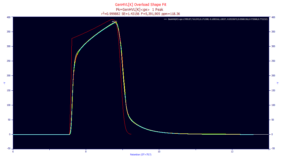
The above GenHVL[K]<ge> fit successfully uses the <ge> IRF to capture the extensive tailing from the overload state. In this example, there is a significant increase in the 'e' exponential component to manage the tailing. The red curve is the IRF deconvolved peak. With the fitted <ge> IRF absent, the red peak looks quite similar to a [K] shape as in the prior plot's first collection of examples. In general it will be the exponential in the <ge> IRF (or the larger exponential in the <e2> IRF) that captures the extensive tailing.

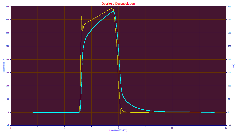
For overload shapes, IRF Deconvolution will be challenging, even when the precise <irf> parameter values are known from a successful fit. It may not be possible to perfectly remove such large IRF's by Fourier deconvolution prior to fitting. Deconvolution adds noise to a signal, and the Fourier filtration may be critical with respect to signal-noise thresholding. You may need to experiment with different filtration levels and methods to best recover the deconvolved shape from the fitting.

Even when using fitted IRF values, an IRF deconvolution of an overload shape is not likely to recover the fitted deconvolved shape absent artifacts of the Fourier discrete processing of the data. In the above deconvolution, the exact IRF from the fitting in the GenHVL[K] fit is used with close to an optimal Fourier domain noise filter. If you see these visually unwelcome oscillations, don't assume such shapes cannot be fitted in PeakLab. You will probably need to set the amplitude threshold to 100% (this always ensures a single peak). If the local perturbations in the data are small enough you may also be able to remove them as a source of peak assignment by increasing the smoothing in the placement algorithm. So long as the Fourier induced oscillations in the time domain offset (no significant bias was introduced in the deconvolution), a successful fit can be made.

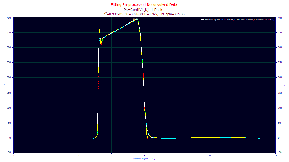
It may not be especially elegant, but in this example, the fit of the pre-deconvolved data is surprisingly accurate:

These are the non-IRF parameters from the GenHVL[K]<ge> fit:

499.870445        7.61242713        0.17130828        -0.1003158        1.00369525        -0.0533672

These are the parameters from the GenHVL[K] fit after the deconvolution preprocessing:

499.713295        7.61435193        0.17217918        -0.1000960        1.00565811        -0.0534377

The differences in the parameters are small as the Fourier-domain induced oscillations in the time domain data are local enough to present little bias in the fitting. The fit error will always be higher when fitting pre-deconvolved data versus the much slower fitting of the raw data with the model containing the <irf> convolution integral. In this instance, the error with fitting the deconvolved data is appreciably higher (715 vs. 118 ppm unaccounted variance), but the deconvolved shape from the <irf> fit is essentially fully recovered.

The GenHVL[K] model is part of the unique content in the product covered by its copyright.