PeakLab v1 Documentation Contents            AIST Software Home            AIST Software Support

Modeling Spectra - Part III - Field Site NIR Data

Authors: Amruta Behera¹ (amruta.behera@plaksha.edu.in), Hasika Suresh² (hasika.suresh@tufts.edu), Rudra Pratap³ (rudra.pratap@plaksha.edu.in), Ron Brown⁴ (ron@aistsoftware.com)
Publish Date: January 2023.

¹Amruta Behera is a founding professor at the new Plaksha University in Mohali, the planned city in the Punjab near Chandigarh, India. Amruta managed the project where the data shown in this white paper was generated as part of his several years of post-doctoral research at the Indian Institute of Science (IISc) in Bangalore, India. In this project, handheld spectrometers were designed, built, and tested for in-field analysis of spices and other cultivated botanicals.

²Hasika Suresh is a doctoral student in the department of Chemical and Biological Engineering at Tufts University, Boston. While she was at the Centre for Nanoscience and Engineering (CeNSE) at IISc India, she developed the HPLC methodology for curcuminoid and turmeric samples and worked to procure a vast library of turmeric roots and powders. Hasika generated all of the chromatographic data illustrated in this white paper.

³Rudra Pratap is the founding vice chancellor (president) of Plaksha University. Prior to this position, Rudra served as the Deputy Director of Indian Institute of Science, Bangalore, India where he founded of the IISc Centre for Nano Science and Engineering (CeNSE) and where, for a time, he served as chairman of the board of a major scientific and statistical software company. In an effort to create tools for Indian farmers growing spice crops to better quantify the value of their harvests, Rudra created and guided the R&D project that resulted in all of the chromatographic and spectroscopic data that appears in this series of modeling white papers. The samples analyzed in these white papers were collected across several years and now represent what we believe to be the most comprehensive and diverse library of commercially grown turmeric in the world.

⁴Ron Brown is the founder of AIST Software, in Oregon, USA, and the author of the PeakLab software, as yet unreleased, which was used to analyze much of this data that appears in these white papers. Ron developed the original PeakFit software and also authored the TableCurve software products for curve and surface fitting as well as AutoSignal for signal analysis.

NIR Field Site Spectral Modeling

In this third white paper in this spectral modeling series, we will demonstrate NIR spectral modeling of the total curcuminoids in turmeric powders using the spectra generated by proprietary handheld field-site spectrometers. Such devices were developed by authors 1 and 2 as part of a grant carried out at the CeNSE labs at the Indian Institute of Science, Banglaore, India. The project involved the novel design of small handheld spectrometers that could furnish an immediate feedback of turmeric quality, the concentration of total curcuminoids and components, as well as using the NIR spectral information to estimate the moisture content in the powder at the time the analysis was being carried out.

You will definitely want to review the Modeling Spectra - Part II - FTNIR Data white paper prior to this one. It illustrates many of the basics associated with modeling powder spectra in the NIR band. To appreciate the chemistry and the HPLC component of the modeling, you may wish to review the Modeling Spectra - Part I - UV-VIS Data white paper.

In the following white paper we will discuss many of the advanced modeling issues encountered in designing and testing an inexpensive handheld spectrometer where samples will be analyzed outside of a controlled laboratory environment, and where the spectral resolution will be appreciably less than that observed in the state of the art FTNIR powder spectra used in the Modeling Spectra - Part II - FTNIR Data white paper.

Computing the Instrument Response Function for the Handheld Device

There are a variety of ways to determine spectroscopic resolution. We are fortunate in having the very high resolution of the FTNIR spectra Of Part II as a reference point. We can estimate the more limited resolution of non-Fourier NIR laboratory spectrometers and that of handheld NIR detectors using the FTNIR resolution as a starting point. We smear or broaden the FTNIR data with a symmetric two-sided Gaussian convolution until this artificially broadened FTNIR data approximately matches the broadening in the device being studied.

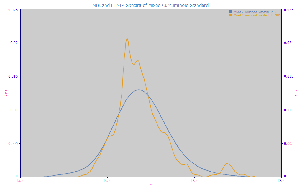
Since the laboratory NIR spectra was especially weak in resolution, we will not describe the instrument's specifics other than to note that this is a widely-used benchtop NIR spectrometer. The following plot compares the NIR 1600-1850 nm spectra of the mixed curcuminoid standard in the FTNIR with a traditional lab instrument NIR spectra.

Fig. 1 Comparison of NIR 1600-1850 nm Spectra of Mixed Curcuminoid Standard using FTNIR and a Conventional Laboratory Instrument NIR

The FTNIR is in the amber, the conventional NIR in blue. We used a genetic algorithm to increase the Gaussian SD convolution width (PeakLab, IRF Deconvolution option) until the attenuation (amplitude decrease) of the convolved FTNIR data matched that of the blue curve on an area normalized basis. Since the same material is being analyzed in both spectra, we should be able to approximately reproduce the blue curve by this additional Gaussian smearing - if the only difference between the instruments is the much higher resolution of the FTNIR.

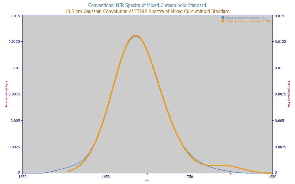
Fig. 2 The NIR data as measured and the FTNIR data with an added 18.5 nm SD two-sided Gaussian convolution

We were able to come very close to matching the shape by a Gaussian broadening of the FTNIR data. The wavelengths did not perfectly match, however. We also had to shift the conventional NIR spectra +4 nm to see the alignment shown above. Since the broadening in a Gaussian by a Gaussian IRF is such that final width will be the sqrt(wid₁² and wid₂²), the square root of the sum of the variances, and since we believe the estimated Gaussian line broadening or IRF of the FTNIR will be close to its fitted Gaussian SD a₂ widths in the Part II peak fits, about 4 nm, the estimated line broadening or IRF for the conventional NIR spectrometer can be estimated at sqrt(4²+18.5²) or 18.9 nm.

The Impact of Resolution on Modeling

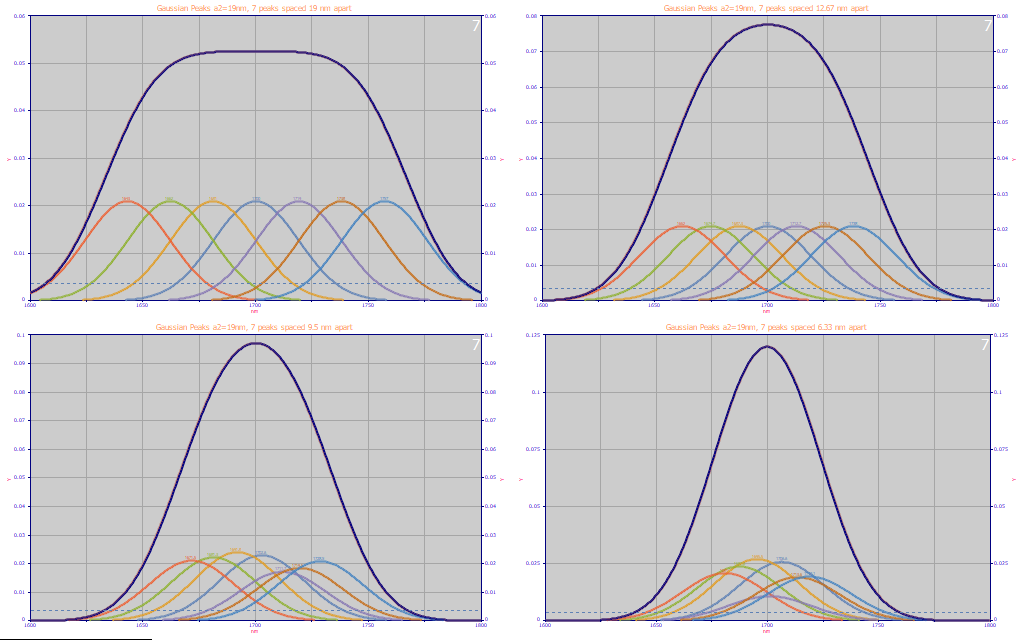
Fig. 3 Seven 19nm width Gaussians spaced 19nm 12.67, 9.5, 6.33 nm apart

In Part I and Part II of this white paper series, we mentioned a rule of thumb we use for modeling where we see no value in a wavelength spacing of predictors any smaller than about half the estimated Gaussian width of the components that can be fitted to any spectral feature. Fig. 3 above illustrates this in a manner that is readily understood. We generated data consisting of 7 equal amplitude Gaussians each with 19 nm a₂ (SD) widths and spaced them apart by 1 SD (19 nm), 2/3 SD (12.67 nm), 1/2 SD (9.5 nm), and 1/3 SD (6.33 nm). No noise was added. We wanted to see where the fitting would break down. The 2/3 SD resolves the peaks at both amplitude and wavelength. At 1/2 SD (9.5 nm) the amplitudes and wavelengths can no longer be completely resolved, even with full-precision data. It is appreciably worse at 1/3 SD (6.33 nm).

Based on this analysis, we can say that a 10 nm spacing is fine were we to model NIR spectra from this benchtop laboratory NIR instrument.

Peak Fitting Benchtop NIR Spectra

Fitted Parameters

r² Coef Det      DF Adj r²      Fit Std Err      F-value      ppm uVar

0.99999759      0.99999753      0.00016500      17,396,636      2.40604220

 Peak      Type       a0       a1       a2

    1      Gauss      0.69437174      1611.32129      17.1690077

    2      Gauss      3.28294153      1649.36996      17.1690077

    3      Gauss      9.55528456      1672.78305      17.1690077

    4      Gauss      10.2210843      1695.43333      17.1690077

    5      Gauss      4.81623486      1719.46706      17.1690077

    6      Gauss      1.39663472      1747.94205      17.1690077

    7      Gauss      0.39725356      1780.12448      17.1690077

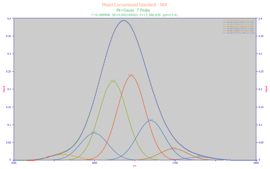
Fig. 4 Peak fit of equal-width Gaussians to the NIR data

In Fig. 1 of part II of this white paper series, we fit this same mixed curcuminoid standard's FTNIR data to equal-width Gaussians. That fit required 27 Gaussians and each was 3.6 nm in a₂ width. While useful for an FTNIR model, we accept that we will have a much weaker resolution with conventional NIR spectral data. As a confirmation of the spectral broadening and to estimate the expected wavelengths, we fit the lab instrument NIR to a sum of equal-width Gaussians. In the Fig. 4 fit, we found that a fit to 7 peaks was what was needed to get in the vicinity of 18 nm peal widths.

When a mix of absorbances are highly smeared, as occurs here with this conventional NIR spectrum, only a single peak is observed instead of the many peaks apparent in the FTNIR spectra of this same sample (Fig. 1). This level of convolution makes it very difficult for the peak fitting algorithm to determine the width of the components by an F-statistic type of optimization. Here we only note that there is a very strong 1672 and 1695 nm peak.

Handheld NIR Spectrometer Resolution

For the next step, we estimated the instrument response broadening from two different micro-NIR sensors which were integrated into custom handheld NIR turmeric powder spectrometers.

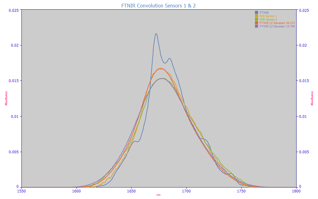
Performing that same type of Gaussian convolution to produce matched attenuations of the FTNIR data, we were pleasantly surprised to learn that these handheld sensors offered considerably higher resolution than our conventional NIR benchtop spectrometer. Sensor 1's spectrum of this mixed curcuminoid standard is the amber curve, the red curve a Gaussian convolution of 10.2 nm producing a matched attenuation. Sensor 2's spectrum of this mixed curcuminoid standard is the green curve, the lavender curve a Gaussian convolution of 13.7 nm producing the matched attenuation. In both cases, the resolution of the handheld NIR sensors were appreciably better than the 18.5 nm convolution that was needed for the benchtop instrument.

With a known FTNIR Gaussian width of 4 nm, the Type 1 sensor's Gaussian SD line broadening is sqrt(4²+10.17²) = 10.93 nm

With a known FTNIR Gaussian width of 4 nm, the Type 2 sensor's Gaussian SD line broadening is sqrt(4²+13.75²) = 14.32 nm

While neither handheld sensor could match the exceptional 4 nm peak width resolution seen with the FTNIR, the 10.9 nm sensor's resolution is a dramatic improvement over the 18.9 nm resolution NIR lab instrument spectra. All else being equal, Sensor 1 would be the clear choice for the handheld device. From this analysis, and our rule of thumb for modeling, a 5 nm wavelength spacing is reasonable for modeling Type 1 NIR spectra.

S/N considerations

For a given resolution, we would prefer a handheld spectrometer that offers the highest possible Signal/Noise ratio.

The S/N in a spectrum will be impacted by the optics and electronics in the device, by the digitization, and by the software, especially if there is any subsequent averaging of multiple measurements. The measurement of S/N is equally complex. For this data, we used PeakLab's time and Fourier domain S/N estimates. The time domain uses a cubic accuracy interpolant to estimate deviations that map to a white noise model. The Fourier domain method assumes that only noise exists at the highest frequencies (a very good assumption with data consisting of spectral peaks), and the 'noise floor' at these higher frequencies directly furnishes an estimate of where all precision is lost in the data. S/N can be reported as a noise fraction (often ppm), as significant digits of precision, or in decibels where a difference of 20 represents 1 order of magnitude.

Fig. 6 PeakLab analysis of S/N for the modeling data spectra in Parts 1-3 of this white paper series

The time domain analysis of S/N reports the estimated white noise in ppm in the first column above, the corresponding level of noise in decibels, and the significant digits where there is just 10% noise, where there is 50% noise, and where there is 90% noise. The Fourier portion of the analysis will give the db noise floor (the power spectrum value at the highest frequencies) and also an estimate of the significant digits where all precision has been lost, where all information represented in the data values is noise.

The UV-VIS spectra used in the Part I of this white paper series has a weak S/N, but we note that these spectra yielded a superb prediction accuracy in the total curcuminoid models. The FTNIR spectra used in Part II of this series has a much stronger S/N, but we saw weaker model predictions, which we attributed to the additional complications of powder measurements and a considerable measure of obfuscating absorbances in the NIR bands. In the two handheld NIR sensors, which also process powders, we will see the same issues as seen in the FTNIR models. Still, we can make the leap that if 2.26 significant digits was enough for a successful model in the UV-VIS spectra, the 2.70-2.80 digits of precision should be sufficient for the handheld NIR spectra.

In our experience, if the errors (residuals) in fitting are normally distributed, the fitting process will manage noise with little adverse impact upon the quality of the prediction estimates in the fitted models. In other words, with a large body of modeling data, the residuals in the fitting may well offset one another, and this may occur with errors in both the Y reference data and in the X predictor spectra. This is also why data are rarely pre-smoothed in any form of regression analysis.

Peak Fitting the Average Turmeric Spectrum - Type 1 Sensor

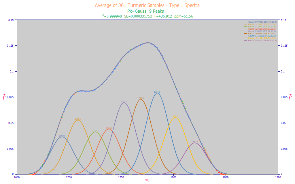
Fitted Parameters

r² Coef Det      DF Adj r²      Fit Std Err      F-value      ppm uVar

0.99994844      0.99994601      0.00033175      436,912      51.5623761

 Peak      Type       a₀       a₁       a₂

    1      Gauss      0.99720088      1693.47805      10.9000000

    2      Gauss      1.44087633      1708.65130      10.9000000

    3      Gauss      1.12921695      1725.23981      10.9000000

    4      Gauss      1.20515221      1738.22795      10.9000000

    5      Gauss      1.90615668      1752.91978      10.9000000

    6      Gauss      1.99231168      1768.90317      10.9000000

    7      Gauss      2.15964675      1784.62249      10.9000000

    8      Gauss      1.51196564      1801.72915      10.9000000

    9      Gauss      0.84010088      1820.57542      10.9000000

Fig. 7 PeakLab Gaussian peak fit of average spectrum from all Type 1 Spectra

We know from the experiment plotted in Fig. 3, that we will lose the capacity to accurately fit peaks spaced closer than 1/2 of the IRF, or about 6 nm. We have no issue with such narrow spacings in the fit that produces this 10.9 estimated peak width. This occurs with 9 Gaussian peaks. The fit is weaker, but we expect some of that from the higher noise in the Type 1 spectra.

The a₁ Gaussian center values in Fig. 7 represent a fair starting point as to the wavelengths likely to be found by a multivariate linear modeling algorithm.

Direct Spectral Fit of Total Curcuminoids - Sensor 1

We will now begin the actual spectral fitting. We will use a 5 nm spacing, 1650 -1850 nm, with a final refinement to 1 nm. At this predictor density, it was possible to fit all permutations through 8 predictors without using any form of filtering. Every possible permutation 1-8 predictors was fitted. The total fitting time was a little over 1 minute.

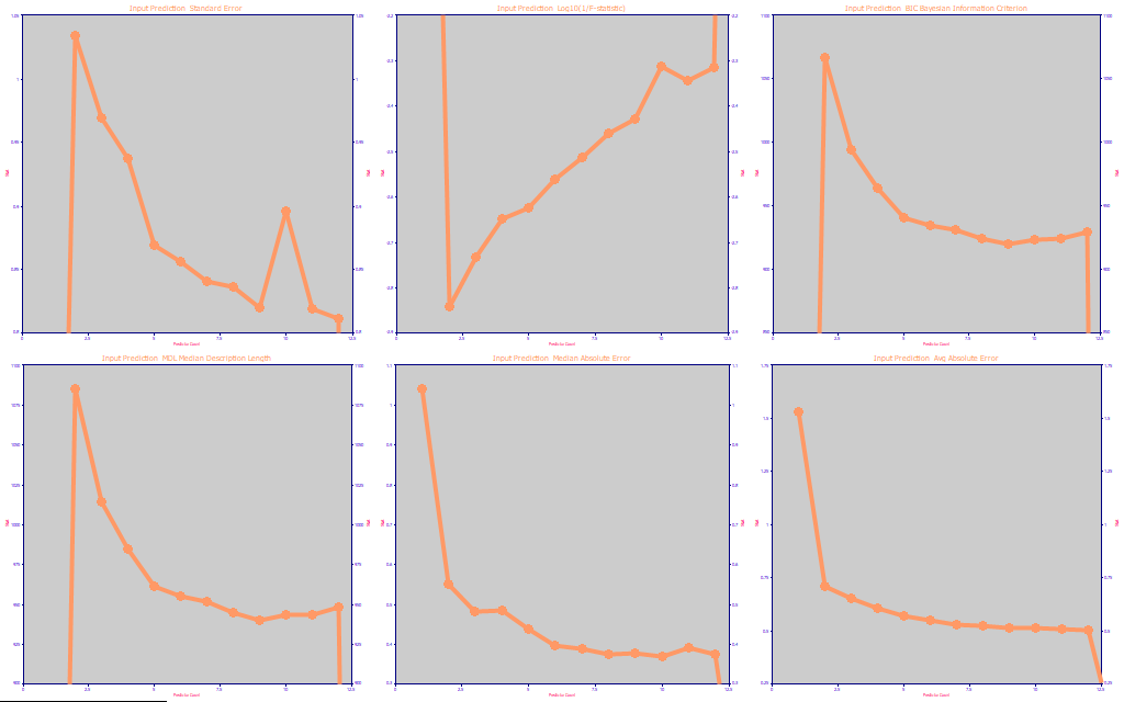
Fig. 8 The prediction optimization statistics for the modeling, average of the five best retained models at each predictor count

We use the same type of prediction optimization we discussed in Part I and Part II of this white paper series, the SE, an inverse form of the F-statistic, the BIC (Bayesian Information Criterion), the MDL (Minimum Description Length), the median prediction error, and the average prediction error.

The optimum predictor count by SE is 12. By the very conservative F-stat, it is just 2. These are the two metrics most often used by statisticians in least-squares modeling. We look mainly at the next four panels where the BIC reports an optimum of 9, the MDL an optimum of 9, the median error an optimum of 10, and the average error an optimum of 12. There are no individual fitted models beyond 12 since this was a maximum set at the time of the fitting.

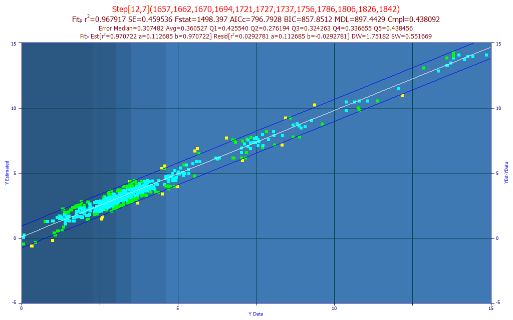
Fig. 9 The model plot for the best 12-predictor total curcuminoids model by average prediction error

The data was meticulously hand-cleaned to remove samples where the chromatography and/or spectroscopy replicates were inconsistent or human error occurred. The data was also extended with samples from drying and humidity chamber experiments to help teach the modeling algorithm how to interpret moisture differences. There were also spent turmeric spectra (nearly all of the curcuminoids removed) to help the modeling algorithm know where the zero should be. The predicted rČ is 0.968 (leave one out), higher than the 0.941 seen with the FTNIR 7-predictor model in Part II of this series, but the rČ will vary with the distribution density of the Y-values. Here we will look at the average prediction error, a much more robust estimate of error, as our reference. Here we have an average prediction error of 0.361 total curcuminoid percent, as compared to the 0.285 in the FTNIR powder models and 0.113 in the UV-VIS liquid model.

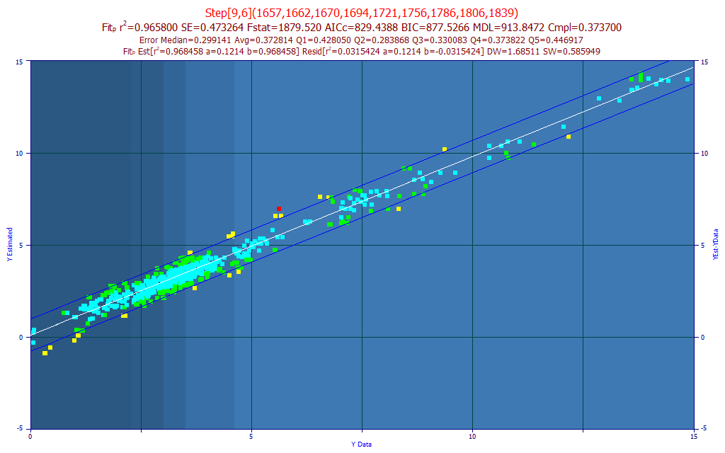
Fig. 10 The model plot for the best 9-predictor total curcuminoids model by average prediction error

If we assume the optimum model follows the BIC and MDL information criterion, we would select a 9-predictor model such as the one above. The median error is actually lower than the 12-predictor model, although the average prediction error is slightly higher, .373 instead of .361.

In using PeakLab's 'stepwise' models, those beyond the full permutation upper limit of 8 predictors, we are no longer in that zone where we see every possible model. We are at the mercy of the advanced search algorithm in this procedure that uses a given full-permutation model as its starting point. In the 12-predictor model above, a 7-predictor full permutation model was expanded by 5 additional predictors. In the 9-predictor model, a 6-predictor full permutation model was expanded by 3 additional predictors.

PLS Spectral Fit of Total Curcuminoids - Sensor 1

We ran a PLS (partial least squares) reference (NIPALS, Systat, Leave One Out prediction errors). The fit used a 1 nm spacing from 1650-1850 nm to match the 1 nm resolution we realized in the Fig. 9 and Fig. 10 direct spectral fits. There are thus 201 PLS wavelengths, (202 parameters). The optimum prediction rČ occurred with 11 factors, 0.9517 (48,300 ppm statistical error). In the Fig. 9 and Fig. 10 direct spectral fits, the 12-predictor model has a 32,100 ppm error and the 9 predictor model a 34,200 ppm error.

In Unscrambler, 1 nm spacing, the NIPALS PLS also gave the best leave-one-out rČ of prediction at 11 factors, 0.9528 (47,176 ppm error). For the PCR modeling, the best leave one out predictions were seen with 8 principal components, rČ prediction 0.9374 (62,552 ppm error). we again note that we have never seen a PLS or PCR model match the prediction of the best performing direct spectral fits.

We also ran a PLS reference from 1550-1950 nm. The additional 100 nm to each side of the 1650-1850 nm modeling band was added to include moisture band signal. We wanted to see if the moisture correlations would produce stronger or weaker total curcuminoid PLS predictions. The curcuminoids, especially curcumin, have almost no water solubility and turmeric powders with high curcuminoid content consistently have less moisture takeup. We are strong advocates of not using indirect or inferential predictors, but we did want to see how a PLS model treated this secondary moisture information. For this reference, the PLS fitting optimized (leave one out) to a 12-factor model with an rČ of prediction = 0.9501.

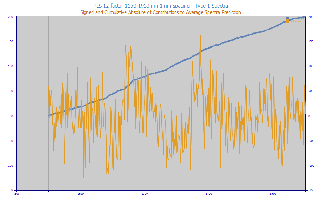
Fig 11. The PLS contributions to the average turmeric spectra estimate. 1550-1950 nm, 1 nm spacing, 12-factors

In Fig. 11, we plot the value at each WL that goes into the prediction for the overall average type-1 spectra using this optimal 12-factor 1550-1950 nm PLS model. We see the 401 contributions to the 3.8578 % total curcuminoids predicted value. Certain WLs add over 100% percent total curcuminoids to this prediction estimate, others subtract over 100%. The water band information, which we know is only indirectly correlated with the curcuminoids, makes up nearly half the absolute model estimate contributions shown in the blue curve (1550-1650 and 1850-1950). The blue cumulative curve was normalized to 200 in order to overlay the raw data.

Direct Spectral Fit of Moisture Levels in the Turmeric Powder - Sensor 1

To fit the moisture level in the turmeric powder, we must include the water bands. The handheld NIR sensors cover 1550-1950 nm. The 1900 nm water band is thus included as well as the tail of the very strong 1450 nm band. We thus fit 1550-1950 nm at 5nm spacing using the default filters to speed the fitting. The estimates without using the default filters are for 36 billion fits and 5.8 hours. With these filters, there are 14.5 million fits and 9.1 seconds.

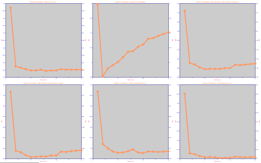
Fig. 12 The prediction optimization statistics for the moisture modeling, the best retained model at each predictor count

The optimization is a consistent 5-predictors across all metrics except for the F-statistic.

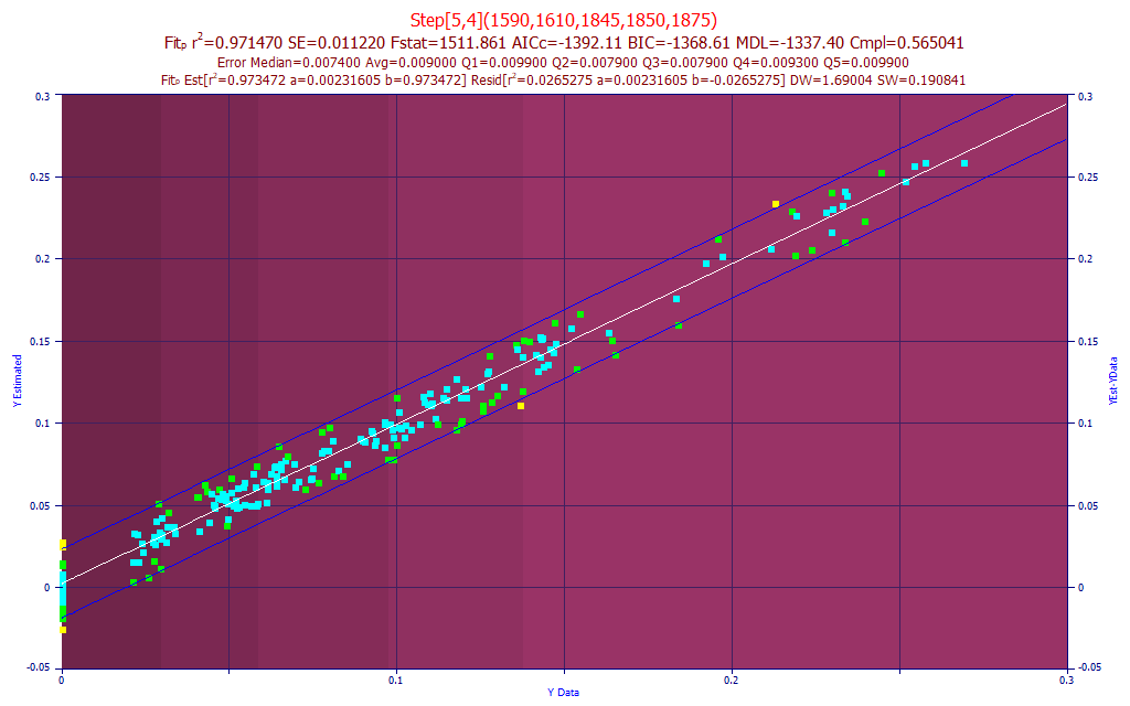
Fig. 13 The model plot for the best 5-predictor moisture model by average prediction error

This is what we wanted so see. Despite the whole of the curcuminoid modeling band being available to the modeling algorithm, only water band wavelengths were selected in the best retained fits. The moisture data varies from 0.00 to 0.27 (0 - 27%), and the average absolute error is 0.009 or 0.9%. The large number of points at 0 are from the spectra of oven-dried samples cooled in a desiccator before being run and these data were assumed to have zero moisture.

For a PLS reference, we fit the whole 1550-1950 nm modeling band, 5 nm spacing, just as was done for the direct spectral fit. In Unscrambler, the program chose a 4 factor model as the optimum with a leave one out rČ of prediction of 0.9517. If we run out to 9 factors, however, we see 0.9711. For a PCR reference, Unscrambler chose 4 principal components as the optimum with a leave one out rČ of prediction of 0.9501. If we run out to 9 principal components, we see 0.9680. At a 5nm spacing, these PCLS and PCR models have 81 predictors, 82 coefficients. The simple -predictor direct spectral fit achieves the same or better prediction accuracy with six coefficients.

Direct Spectral Fit of Total Curcuminoids - Sensor 2

Given the preliminary analysis of resolution, we would not have expected the sensor 2 models to be as effective. For this data. most of the optimization metrics flattened at or near 12-predictors.

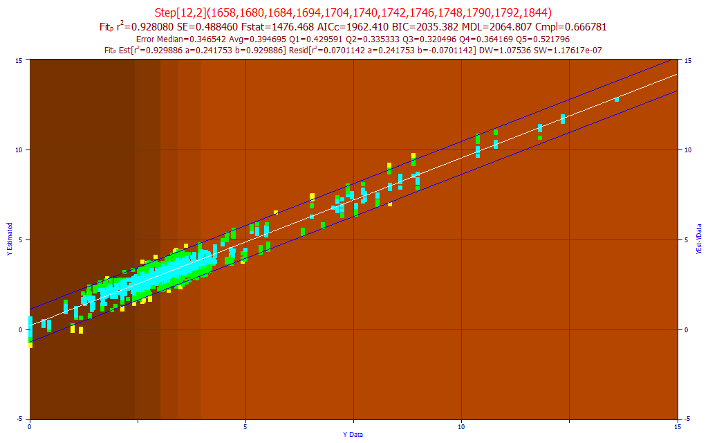
Fig. 14 The model plot for the best 12-predictor total curcuminoids model by average prediction error - sensor-2

For this data, we show all replicates fitted. We have found this a useful method for quickly spotting outliers in the spectra replicates. If we look at the average error, we find 0.394 (12-predictors) as compared to 0.361 for the sensor-1 12-predictor model. The weaker resolution (the higher IRF spectral line broadening) made the fitting more challenging and the overall average prediction error is about 10% higher.

Direct Spectral Fit of Component Curcuminoids - Sensor 1

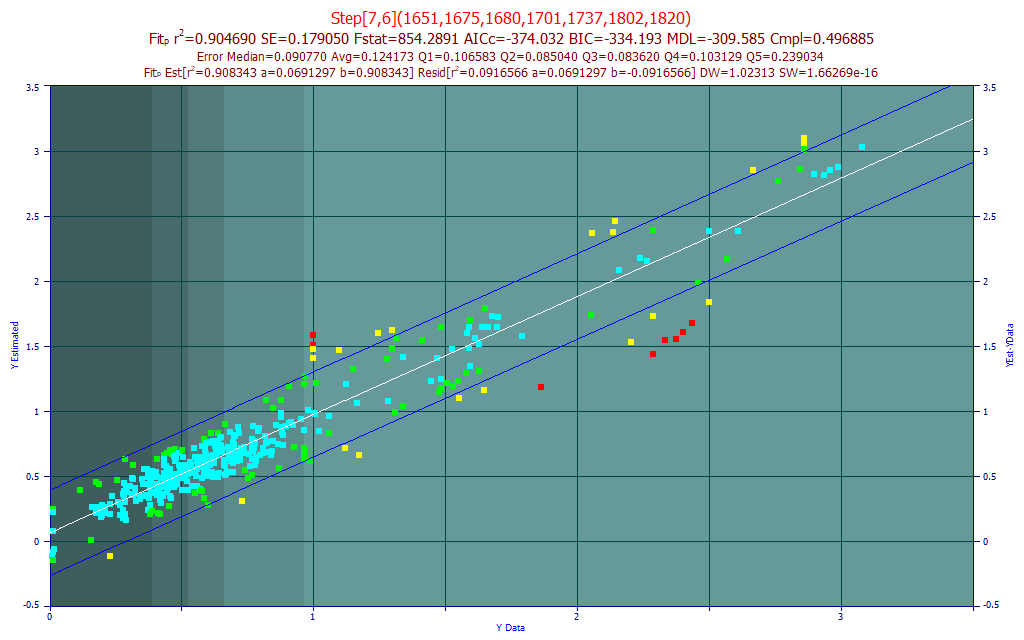
Fig. 15 The model plot for the best 7-predictor BDMC component model by average prediction error - sensor-1

The BDMC fit is weaker. The BIC and MDL suggested little benefit beyond 7-predictors. Here the average prediction error is less, .124%, but the BDMC values range from 0-3%. Clearly there are certain turmeric samples where the model is struggling.

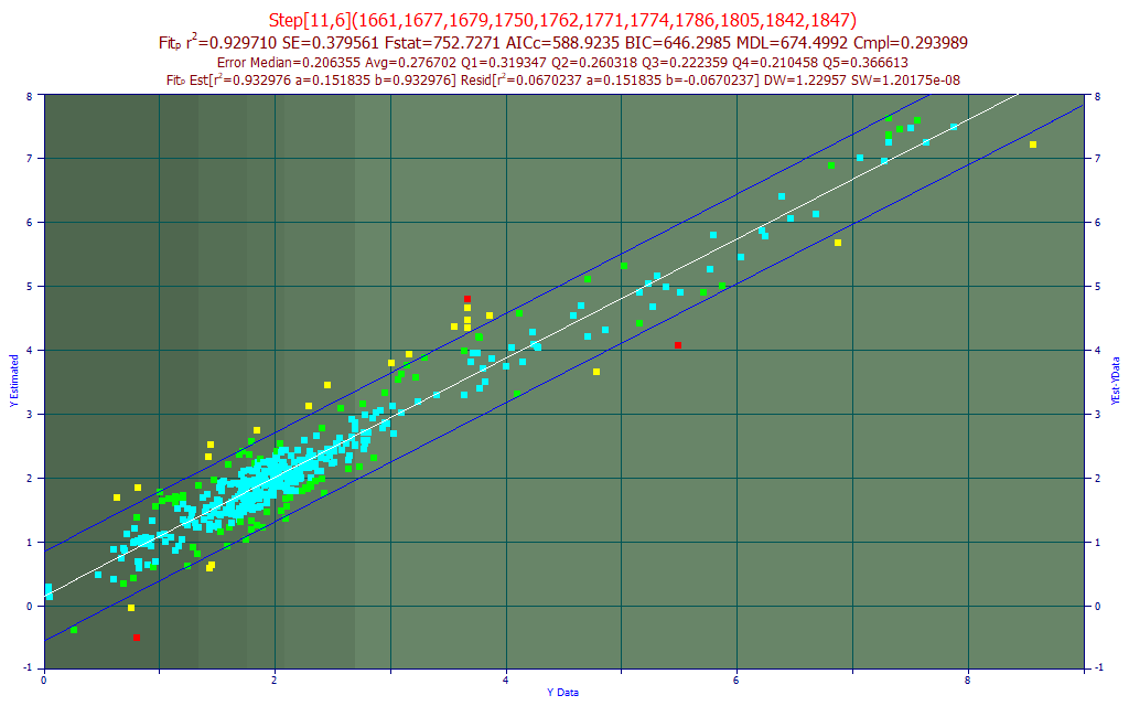
Fig. 16 The model plot for the best 11-predictor curcumin component model by average prediction error - sensor-1

The curcumin component fit is better. The BIC and MDL optimized to 11 predictors. The average prediction error is .277%, with the curcumin ranging up to 8%.

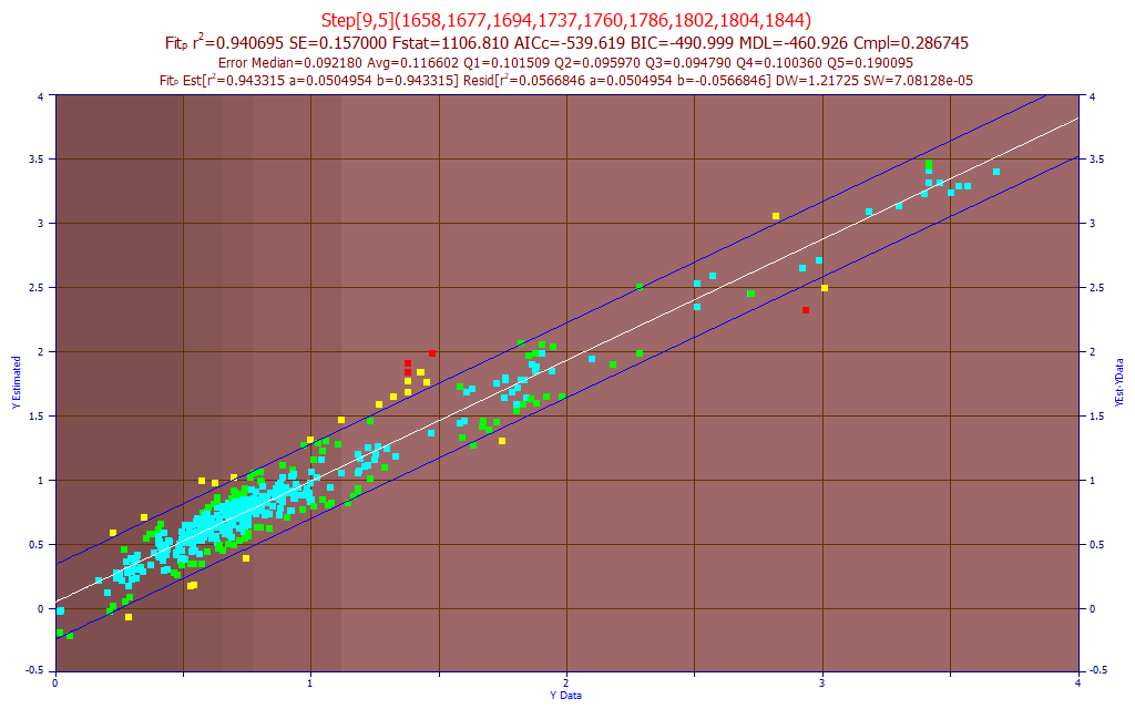
Fig. 16 The model plot for the best 9-predictor DMC component model by average prediction error - sensor-1

The DMC component fit is actually quite good. The BIC and MDL optimized to 9 predictors. The average prediction error is .117%, with the DMC ranging up to 4%.

Spectral Modeling

We hope these spectral modeling white papers have offered a beneficial illustration of building US-VIS and NIR models using direct spectral modeling.