PeakLab v1 Documentation Contents AIST Software Home AIST Software Support
White Paper: Part II - Chromatographic Models and IRFs
Part II - Chromatographic Models and Instrument Response Functions
In Part I of this series we described a generalization of the HVL and NLC chromatographic models which accommodated higher moment differences in the zero distortion (infinite dilution) density underlying the peak shapes in chromatographic separations. In that discussion we alluded to the importance of accounting the additional nonidealities in the chromatographic flow and detection systems, but used data where these instrumental distortions were removed prior to fitting. In Part II of this series of white papers, we will cover the benefits of modeling these instrumental and system distortions when fitting chromatographic data.
Instrument Response Functions and Convolutions
To understand instrument response functions (IRFs), in chromatography, it is useful to look at the convolution science for the peaks observed in spectroscopy.

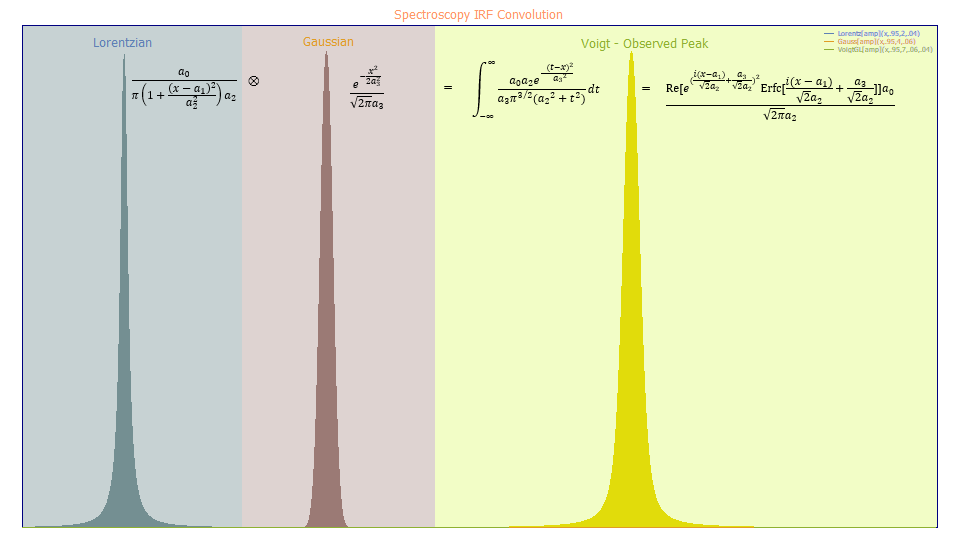
The natural spectral line is not a pure line, or delta signal, but rather a spectral line broadening that typically has a Lorentzian line shape. By spectral broadening theory, this shape arises from both natural and collision effects. In the real world, the true line shape, must be processed using an instrument whose optics introduce distortions typically referred to a point spread function. The energy's frequencies will be further broadened by the lenses, mirrors, and other optical elements in the instrument as well as the optics and electronics in the detector. The combination of all of these added distortions or nonidealities is known as an IRF, the instrument response function. In general, the instrumental smearing in spectroscopy will be Gaussian.
The smearing of one density by another is generally described by a mathematical convolution, shown above with the ﺥ symbol. A convolution is an integral, and with respect to two densities, most will not have closed-form solutions. When a Lorentzian is convolved with (smeared by) a Gaussian, the resultant observed peak, as registered by the instrument, is a convolution integral whose shape is known as the Voigt profile, a model whose tails will not decay as slowly as the Lorentzian, but not as fast as the much more compact Gaussian.
In the case of the Voigt spectral peak, there is a closed-form solution, although as shown above, it exists only in the complex domain.
Chromatography and IRFs
The science of chromatography is appreciably more demanding in both the instance of the model for the true peak, that which arises from the chromatographic separation, and in the IRF which involves both the distortions in a directional flow path and a very different detection system. The following example uses actual parameters from real-world chromatographic data fits:
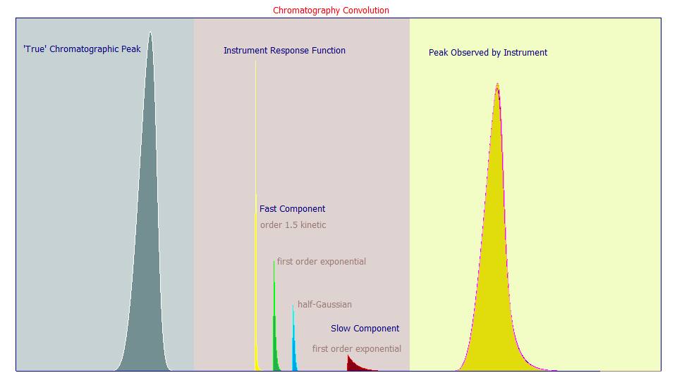
We covered the issue of the 'true' peak model in the first white paper. We now look at the non-chromatographic separation portion of the peak shape reported by the instrument, the IRF or instrument response function.
In the course of our work, we have almost universally observed two components in the IRF of a chromatographic peak. There is a 'fast' component, one of a narrow width with respect to broadening, and a 'slow' component of a considerably greater width. We also found that these two distortions were concurrent, occurring simultaneously, and not an instance where one finished broadened state was further broadened by a subsequent one, and where a separate convolution would be needed to describe the additional spreading of the second component.
We thus convolve the chromatographic peak, usually a generalized HVL or generalized NLC, as described in part I of this series, with a variable area sum of fast and slow IRF components. This convolution integral produces the peak as observed by the instrument.
In the above plot, the narrow IRF candidates are yellow, green, blue, and the higher width component is shown in red. Each has the same area. If you look at the 'true' peak on the left, and then the high width first order exponential IRF (the red IRF component), and finally the observed shapes on the right, you will see that most of the tailing in the observed peak comes from this high-width red component. We have never observed anything other than a first order kinetic model as appropriate for this higher-width IRF component, and we have found this wider IRF component, for a given instrument and column, to be largely constant; nearly independent of the prep, additives, temperature, and solute concentrations.
The narrow IRF component is less clear. We believe the axial dispersion is likely best represented by a one-sided, directional, probabilistic half-Gaussian (the blue IRF component). The interphase mass transfer associated with porous media has a second order component where the overall resistances can be somewhat approximated by an order 1.5 kinetic decay (the yellow IRF component). One can also use a first order exponential for the narrow width component (the green IRF component) as an approximation for both effects (the half-Gaussian decay shape is close to a .5-.6 order kinetic decay) as well as any low width first order mixing. The good news is that the narrow width component has only a small effect on the overall peak shape and the three fast IRF components shown above can be used close to interchangeably in chromatographic modeling. In the above plot, the peaks from each of the three narrow width IRF components almost completely overlay one another (there are actually three observed peaks in the right pane). Statistically, we have never been able to achieve fit significance with more than one of these narrow width models in the overall IRF. Although we have found this narrow IRF component to be somewhat dependent on the prep, additives, temperature, solute concentrations, and retention, because its influence is small on the overall shape, it can generally be treated as common to all peaks in a chromatogram, and often across a wide range of samples and system variables.
The High Width and Low Width Components of a Chromatographic IRF
The higher width component will thus be the predominant determinant of the IRF tailing. The impact of the lower width component on peak shape will be less even when the fraction of this lower width component predominates.
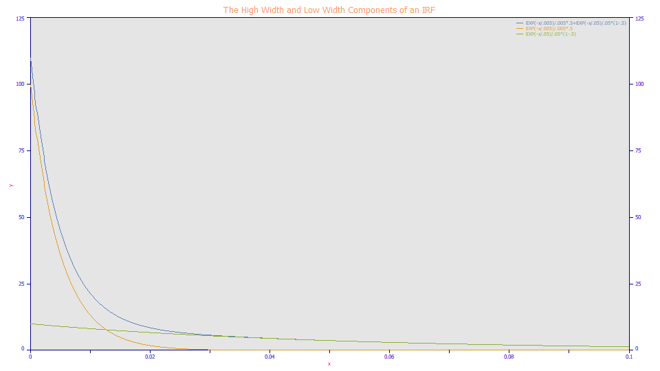
Here we plot a two component two-exponential <e2> IRF and the each of the individual components separately. The fast component governs the decay in the early portion of the curve, and effectively has no influence after a certain point. The slow exponential impacts the shape of the elongated tailing, but not the shape in the fast portion of the decay. The fast amber colored curve and the slow green curve, produce the blue curve, the <e2> IRF. When you look at the IRF-originated tailing within a peak, it is difficult to distinguish the impact of the amber component on the overall peak. Visually, it is mostly the green slow component that is observed.
From the perspective of that which can be successfully estimated statistically, we found that we can only fit a single narrow-width and a single higher-width IRF component. These will be right-sided; all IRF distortions represent delays in the transport or measurement of the solutes. The IRF in a chromatographic convolution model will thus consist of the sum of two discrete (independent) distortions or delays.
One can thus treat the narrow width instrumental distortions as all half-Gaussian based axial dispersion, or all interphase mass-transfer resistances in a 1.5 order kinetic, or in a simplification where all narrow width distortions are also treated as a first order kinetic delay. Each will give an estimate of the quantity of this narrow width distortion and an estimate of the width, but non-linear fitting cannot include and separately quantify different low-width effects. Statistically, the compact half-Gaussian is easiest to fit in the iterative non-linear fitting, the 1.5 order kinetic the hardest since its long sloping decay can start to approximate the slow exponential component of the IRF.
Even though it is possible to treat this impulse-like narrow width component with a good measure of latitude, it cannot be omitted from the IRF. The overall width may be narrow, but the magnitude of this component will be significant. Indeed, we have often found it to predominate in terms of area fraction of the components. Its influence on the overall shape happens to be subtle only because of this impulse-like narrow width.
We will briefly note that convolution models are hardly new to chromatography. If the true peak is treated as Gaussian, and the IRF is a single first order exponential, as in the red curve above, the final peak is an EMG, probably the most widely used chromatographic model historically. We will also note that the EMG is likely to be of dubious value in modern chromatography. We have never observed the true peak to be a Gaussian, or the IRF to be a single exponential, in any real-world chromatographic data set.
Fitting Convolution Integrals
If the peak as reported by the instrument is a convolution of a true peak and IRF, then one must fit this convolution integral in order to deconvolve, to 'unsmear' or separate, the IRF from the instrumental peak in order to report the true non-distorted peak describing the actual chromatographic separation. If the IRF is known in advance, Fourier methods can be used to deconvolve the IRF from the data prior to fitting, as was done in Part I of this series. If the IRF is unknown, it must be determined in some fashion. There are two methods that can be used.
The convolution integral can be fitted to the data and the parameters of the fitted model will give this separation, including each of the parameters describing the IRF. While this can be done using integral algorithms in the time domain, the computation cost will be prohibitive, even with modern computers. A time-domain nonlinear fit using an integral directly could require an overnight computation if the count of data points were high and there were multiple peaks in the data set. The solution is to fit the convolution integrals in the Fourier domain, where convolution and deconvolution are as straightforward as complex multiplication and division. This will enable the fitting of convolution integrals to be done in minutes or seconds as opposed to hours. While not immediate, the fitting can be remarkably fast, and once a given IRF is known for a given column, prep, and instrument, additional convolution integral fits will not be needed except to check on column/system health or in determining the effects upon the chromatographic separation arising from changes in the prep.
Since the IRF parameters will produce a known shape with respect to the deconvolved or sharpened peak, there are also genetic algorithm optimizations that can be done to quite swiftly estimate the IRF parameters. This will be a completely independent method which can be used to confirm IRF fit estimates when these parameters may be correlated with other parameters within the convolution model.
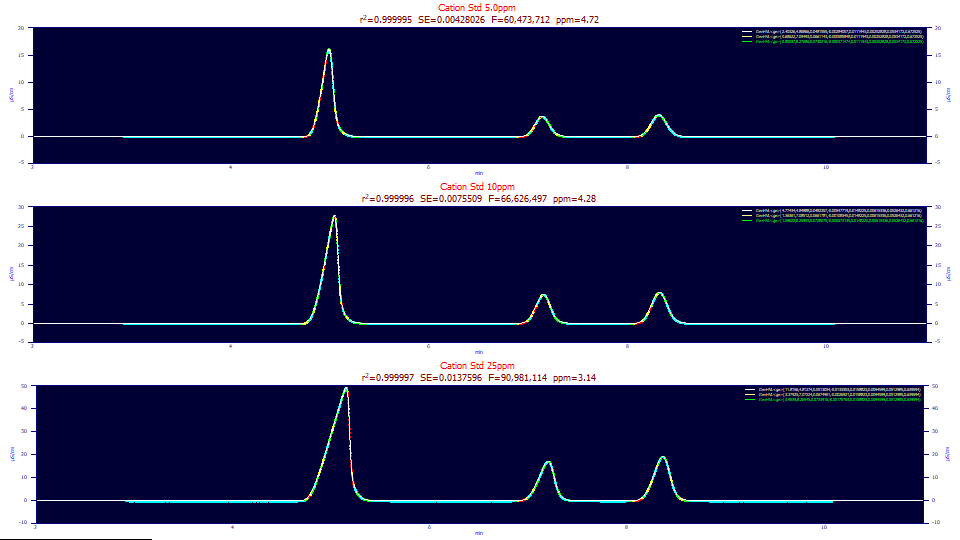
If we fit the baseline-resolved cation standards in the IC data used in Part I of this series to a convolution model, we will see a fit with sub-10 ppm error:
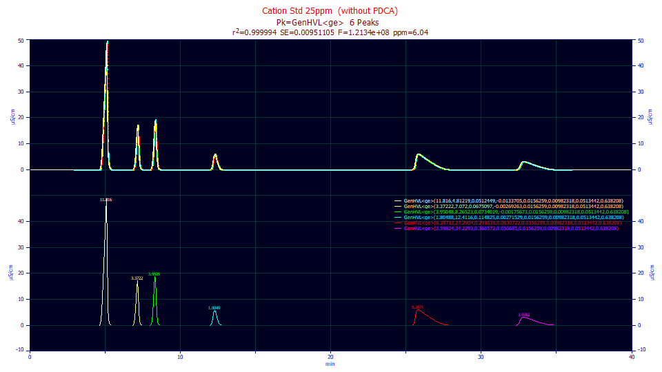
Here we fit with this data set of close to 20,000 data points to a GenHVL (once-generalized HVL) bearing the <ge> IRF, the workhorse IRF containing the sum of half-Gaussian and exponential components. Fitting this data with the Fourier convolution integral innovation, even using an advanced multiple-step fitting procedure to ensure proper convergence to the global solution, required only 16 seconds on a basic i7 machine. By contrast, fitting the Fourier pre-deconvolved data to a closed form non-IRF bearing GenHVL, as we did in part I of this series, required 1.6 sec. We actually fit the actual convolution integral in only an order of magnitude's increase in fitting time, but we managed this in the Fourier domain, avoiding the actual time-domain integration.
How great is the computational burden if the convolution integrals are fit in the time domain? If we fit this data set using a very fast custom Gaussian quadrature time-domain integration routine and a user-defined function that reproduces this same model, the fit shown above required 1.27 hours. If we use a custom adaptive quadrature procedure, also quite fast and better at managing discontinuities and singularities in an integrand, this direct integral fit required 7.42 hours - an overnight processing. Contrast either of these direct integral convolution timings with the 16 sec timing of the Fourier domain convolution model fitting. If high accuracy chromatographic modeling requires convolution integrals, as a several experts in the field have long suggested, and such models were explored only with time domain integration, then little imagination is needed as to why decades have passed with so little progress.
Nonlinear Fitting to Determine IRF Parameters
To illustrate IRF determination by fitting of the convolution models, we will again look at the three concentrations of IC cation standards we fit in Part I of this series. In that example, we removed an average estimate of the IRF in a Fourier deconvolution preprocessing step prior to fitting a non-IRF bearing closed-form generalized HVL model. In this case, we will fit all three data sets to a generalized HVL with a convolution model. To maximize the accuracy of the IRF estimates, we will fit only the first three intrinsically fronted peaks in the data so as to avoid any correlation between the tailed peaks and the tailed IRFs.
"Cation Std 5.0ppm (without PDCA)"
Fitted Parameters
r2 Coef Det DF Adj r2 Fit Std Err F-value ppm uVar
0.99999528 0.99999526 0.00428026 60,473,712 4.71828133
Peak Type a0 a1 a2 a3 a4 a5 a6 a7
1 GenHVL<ge> 2.40325625 4.86865866 0.04815555 -0.0028406 0.01119432 0.00252828 0.05341722 0.67252458
2 GenHVL<ge> 0.68621960 7.09492653 0.06611429 -0.0005858 0.01119432 0.00252828 0.05341722 0.67252458
3 GenHVL<ge> 0.80097027 8.27686392 0.07302161 -0.0003715 0.01119432 0.00252828 0.05341722 0.67252458
"Cation Std 10ppm (without PDCA)"
Fitted Parameters
r2 Coef Det DF Adj r2 Fit Std Err F-value ppm uVar
0.99999572 0.99999570 0.00755090 66,626,497 4.28256208
Peak Type a0 a1 a2 a3 a4 a5 a6 a7
1 GenHVL<ge> 4.77433691 4.84888107 0.04823575 -0.0054772 0.01482250 0.00615336 0.05264319 0.66121627
2 GenHVL<ge> 1.36361163 7.08511663 0.06617812 -0.0010834 0.01482250 0.00615336 0.05264319 0.66121627
3 GenHVL<ge> 1.59622064 8.26902711 0.07280754 -0.0006731 0.01482250 0.00615336 0.05264319 0.66121627
"Cation Std 25ppm (without PDCA)"
Fitted Parameters
r2 Coef Det DF Adj r2 Fit Std Err F-value ppm uVar
0.99999686 0.99999685 0.01375959 90,981,114 3.13617217
Peak Type a0 a1 a2 a3 a4 a5 a6 a7
1 GenHVL<ge> 11.8156012 4.81273677 0.05130538 -0.0133353 0.01588229 0.00945990 0.05129855 0.63959391
2 GenHVL<ge> 3.37924868 7.07224397 0.06749511 -0.0026921 0.01588229 0.00945990 0.05129855 0.63959391
3 GenHVL<ge> 3.95389507 8.26544712 0.07339157 -0.0017576 0.01588229 0.00945990 0.05129855 0.63959391
In this instance of fitting the convolution model to the three data sets, we have just 3-5 ppm least-squares error for all three of the concentrations. The parameters a0-a4 are the same, the parameters of the generalized HVL model, but there are now a5, a6, and a7 IRF parameters shared across all peaks as was done with the a4 ZDD (zero distortion density) asymmetry.
As a point of reference, baseline correction errors can contribute upwards of 10 ppm overall error. The sloppiness of fitting an overall baseline that looks linear to the naked eye, but it comprised of small oscillations, to a straight line, can generate up to 100 ppm error. In general, the S/N of most modern chromatographic data will be so good, most of the unavoidable error in a fit will rest with the measure to which the flow and temperature controllers produce small baseline oscillations and how effectively those are corrected. In general, we look for fits with sub-20 ppm error on analytical data with a high S/N.
These 3-5 ppm error fits can be seen as having very close to full accuracy. This does mean that only .0005 % of the variance in the data remains unaccounted in the modeling. In the tables above a5 is the narrow-width half-Gaussian component of the IRF, a6 is the wider exponential, and a7 is the area fraction of the narrow component. Note that the a6 exponential width is nearly constant across concentration. The a7 parameter is also close to constant with a 2/3 area fraction favoring the narrow width component. Here we will only note that the parameter statistics (not shown here) indicate that the a5 narrow width, while significant, is the least accurately determined of the parameters. For the purpose of this example, we use the time scale directly and report the IRF's widths as an SD and exponential time constant in minutes, although in general a retention scale will be used which will be dependent on the system dead time.
In a chromatographic fit, the a4 ZDD asymmetry, and a5-a7 IRF parameters, are generally treated as constant across peaks. The a4 parameter describes the extent to which the peaks deviate from the HVL's Gaussian zero-distortion density, and the a5-a7 parameters describe the overall instrument distortions. We generally see the wider IRF component, a6 here, as an 'instrument' distortion because it is relatively independent of concentration, temperature, and additive levels. We see the narrow IRF component a5, as a 'system' distortion because it is impacted by concentration, temperature, and formulation.
When these ZDD and IRF parameters are shared across peaks, and fits of less than 10 ppm error are realized, it is virtually impossible to fit independent unshared values for these parameters across even fully baseline resolved peaks. There is simply too little unaccounted variance left to model, and some of that may well be small but systematic error in the baseline subtraction.
You will also need average values of the IRF parameters if these are to be used in a preprocessing deconvolution where the data rather than specific peaks are deconvolved.
In both methods for estimating IRF parameter values, the last portion of a peak's decay to a baseline is needed for accurately estimating the parameters of an IRF.
Once these IRF parameters are known from a standard, a Fourier deconvolution using these pre-determined parameters can be applied to any data set, no matter how overlapping or hidden various peaks may be in the data, in order to remove the instrumental/system distortions prior to fitting a closed-form model.
How important is the higher moment ZDD adjustment in the fitting? How important is the IRF's presubtraction or inclusion in the fitted model? In our experience, both are essential if you wish near zero-error fits. In most cases, however, the IRF's influence will be greatest upon the overall goodness of fit. We have found the IRF to be of critical importance. Neglect these real-world non-idealities in flow systems and detectors, and no measure of theoretical modeling of chromatographic shapes can have any great validity. And to account them, a the IRF convolution integral must be addressed in some manner.
Genetic Algorithm Modeling of Optimal IRF Parameters
The generic algorithm approach to IRF estimation is rather easy to understand, but quite difficult to algorithmically implement.
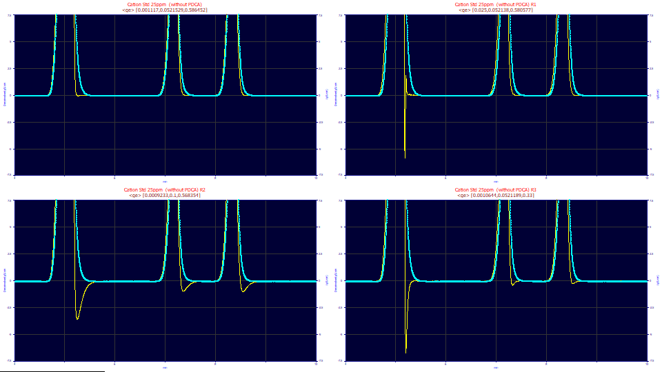
This is the 25 ppm concentration data set, zoomed-in to illustrate the baseline. The blue curve is the instrumental data, the yellow curve various IRF-deconvolutions of the data. No parametric fitting has taken place. In the first panel, the parameters from a genetic optimization of the three <ge> IRF parameters is shown. In the second through fourth panels the half-Gaussian width, exponential width, and area fraction parameters were changed to values well removed from this optimum. You will note that the amount of baseline (within a specified tolerance) is maximized in the first panel's optimization. For chromatographic IRFs, the genetic algorithm adjusts the IRF parameters to seek to maximize the total measure of baseline, minimizing the oscillations which arise from incorrect IRF values.
In this example, the genetic algorithm optimum for this data set and this <ge> IRF consists of parameter values of .0011 for the half-Gaussian SD, 0.0522 for the exponential tau, and 0.587 as the narrow component area fraction. In the convolution model fit above, we fit to 0.0095, 0.0513, and 0.639. The genetic optimization found a much-more impulse-like width for the narrow component, but essentially the same value for the wider exponential component and close to the same area fraction for the components.
The convolution model nonlinear fitting and genetic algorithm Fourier deconvolution approaches for IRF estimation will each have their own advantages and drawbacks. Both require baseline resolved peaks, preferably clean standards with a good S/N and one or more intrinsically fronted peaks.
The convolution fitting is capable of exceptional accuracy, but there can be correlations between the right-shifted ZDD asymmetry and the right-shifted IRF components. especially at low concentrations. Since the distortion operator is a function of concentration, and it transforms the ZDD from a limiting density to a concentration-dependent shape, the higher the concentration, the less these cross-parameter correlations will be present. There is also a practical consideration in Fourier fitting of constraining the widths to keep them high enough in each component to prevent the algorithm from becoming lost at a near-impulse bound where it may be unable to iterate away from these near zero impulse widths.
The genetic algorithm will not get exactly the same estimates when processing the same data because of how it functions with random steps and the massive number of local minima which exist in the optimization problem, but it is not as limited in how small a width may be, and the algorithm, by design, specifies the actual bounds for each parameter. A genetic algorithm optimization will not offer statistical significance of estimates. On the other hand, in a genetic algorithm estimate of an IRF, there will also be no issue of any cross-correlation between the true peak and IRF model parameters since the algorithm processes only the raw data into order to generate a maximum of baseline. This does require a specified tolerance for that which is defined as baseline, and as this tolerance changes, so will the optimized IRF values. Also, deconvolution introduces noise, and subtle changes in the Fourier domain noise filtration, if implemented, will also impact estimated IRF parameter values.
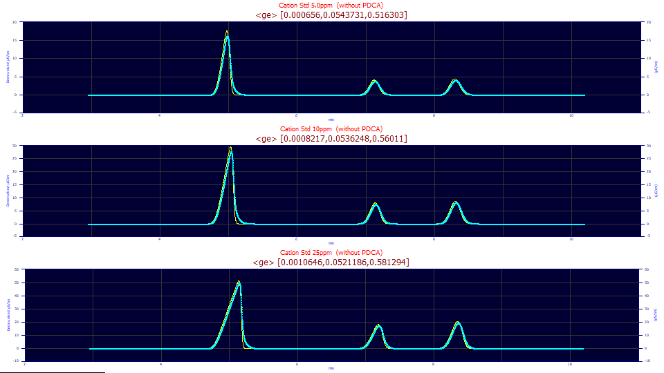
These are the same three data sets which were used in the convolution fitting. The above genetic algorithm IRF deconvolution optimizations remove the instrumental and system distortions using the <ge> IRF model. There is much this type of procedure can reveal about the true nature of an IRF that may be masked somewhat in convolution model fitting. For example, a given IRF may produce especially clean deconvolutions where the peak and baseline meet, but the convolution model with that IRF may not necessarily have the highest goodness of fit amongst various IRF-bearing convolution models. When one is fitting data to very close to zero error, tiny anomalies not covered by the generalized model may be addressed somewhat by a component of the IRF. Exceptional care must be taken when making inferences when comparing fits that are all below 10 ppm error since, in effect, you are making inferences based on the last 0.001 % of the variance in the data.
Here we see GA optimized half-Gaussian widths of 0.00065, 0.00082, and 0.00106 values at the three concentrations. This is about an order of magnitude smaller than the 0.0025, 0.0061, and 0.0094 half-Gaussian widths realized in the convolution model fits. This does illustrate the impulse-like nature of this narrow component and this parametric fitting insensitivity in the narrow-width component. For these data, the x-scale sampling increment is 0.00167 min. The half-Gaussian SDs from the convolution model fits are about 1.5-6x the sampling increment. The half-Gaussian SDs from the genetic optimization are about 0.4-0.6x the sampling increment.
Are these genetic algorithm estimates accurate in their estimating a sharper impulse for this narrow component? If we use this Fourier deconvolution procedure to remove these three IRFs, and then fit the data to the non-IRF bearing closed-form generalized HVL model, we see fits that vary from 7.5-9 ppm error.
"Cation Std 5.0ppm (without PDCA)"
Fitted Parameters
r2 Coef Det DF Adj r2 Fit Std Err F-value ppm uVar
0.99999246 0.99999243 0.00578005 47,747,459 7.54310183
Peak Type a0 a1 a2 a3 a4
1 GenHVL 2.40339444 4.87142437 0.04844772 -0.0028268 0.01058380
2 GenHVL 0.68615567 7.09762529 0.06617236 -0.0005704 0.01058380
3 GenHVL 0.80097096 8.27954058 0.07309052 -0.0003576 0.01058380
"Cation Std 10ppm (without PDCA)"
Fitted Parameters
r2 Coef Det DF Adj r2 Fit Std Err F-value ppm uVar
0.99999220 0.99999217 0.01076029 46,152,175 7.80383272
Peak Type a0 a1 a2 a3 a4
1 GenHVL 4.77478864 4.85510612 0.04901176 -0.0054454 0.01460047
2 GenHVL 1.36283573 7.09066389 0.06634382 -0.0010667 0.01460047
3 GenHVL 1.59622988 8.27450780 0.07296088 -0.0006593 0.01460047
"Cation Std 25ppm (without PDCA)"
Fitted Parameters
r2 Coef Det DF Adj r2 Fit Std Err F-value ppm uVar
0.99999104 0.99999102 0.02416892 40,211,503 8.95672652
Peak Type a0 a1 a2 a3 a4
1 GenHVL 11.8199442 4.82323023 0.05336342 -0.0131590 0.01688233
2 GenHVL 3.37952737 7.08026127 0.06776900 -0.0026668 0.01688233
3 GenHVL 3.95473739 8.27326283 0.07361534 -0.0017421 0.01688233
Clearly, the IRF estimates from this genetic optimization would have to be deemed accurate, as confirmed by this subsequent fitting of the data with the IRF removed. We again note that the GenHVL fit to the uncorrected data had errors of 2578, 2743, and 2353 ppm. Estimating and removing this IRF reduced such error to less than 10 ppm.
Once an IRF has been estimated for an instrument, column, and analysis, the Fourier deconvolution preprocessing requires only a few seconds. Once the IRF has been removed, closed form models can fit large data sets with near immediacy.
We will also note that the IRF quantification is useful for more than recovering the true chromatographic peak. It also quantifies instrument distortions, and those will change as a column ages, fouls, or otherwise suffers diminished performance, or where any aspect of the flow path of the instrument is adversely changed.
Three Chromatographic IRFs
For chromatography data, we have found two other IRFs to consistently perform comparably to the <ge>. The <pe> IRF's narrow component is a 1.5 order kinetic delay to describe a second order step in mass transfer resistances with small porous particles. We repeat the same procedure used with the <ge> IRF with this <pe> IRF model:
"Cation Std 5.0ppm (without PDCA)"
Fitted Parameters
r2 Coef Det DF Adj r2 Fit Std Err F-value ppm uVar
0.99998258 0.99998253 0.00886810 20,490,340 17.4184734
Peak Type a0 a1 a2 a3 a4
1 GenHVL 2.40619788 4.86683284 0.04702743 -0.0028663 0.01478503
2 GenHVL 0.68614184 7.09366769 0.06558237 -0.0006226 0.01478503
3 GenHVL 0.80098021 8.27576450 0.07260047 -0.0004041 0.01478503
"Cation Std 10ppm (without PDCA)"
Fitted Parameters
r2 Coef Det DF Adj r2 Fit Std Err F-value ppm uVar
0.99999068 0.99999065 0.01183994 38,295,760 9.31991780
Peak Type a0 a1 a2 a3 a4
1 GenHVL 4.77818060 4.85240582 0.04802802 -0.0054630 0.01554431
2 GenHVL 1.36277157 7.08863084 0.06602413 -0.0010853 0.01554431
3 GenHVL 1.59617962 8.27269418 0.07270534 -0.0006724 0.01554431
"Cation Std 25ppm (without PDCA)"
Fitted Parameters
r2 Coef Det DF Adj r2 Fit Std Err F-value ppm uVar
0.99999253 0.99999251 0.02217355 47,790,560 7.46829487
Peak Type a0 a1 a2 a3 a4
1 GenHVL 11.8230618 4.82257563 0.05300483 -0.0131776 0.01682157
2 GenHVL 3.37970384 7.07987736 0.06767439 -0.0026727 0.01682157
3 GenHVL 3.95486377 8.27297836 0.07354599 -0.0017450 0.01682157
The <e2> IRF uses a first order exponential for both the fast and slow component:
"Cation Std 5.0ppm (without PDCA)"
Fitted Parameters
r2 Coef Det DF Adj r2 Fit Std Err F-value ppm uVar
0.99999245 0.99999243 0.00580649 47,285,395 7.54808054
Peak Type a0 a1 a2 a3 a4
1 GenHVL 2.40337735 4.87138988 0.04844583 -0.0028269 0.01058693
2 GenHVL 0.68615236 7.09759476 0.06617196 -0.0005704 0.01058693
3 GenHVL 0.80096776 8.27951058 0.07309029 -0.0003576 0.01058693
"Cation Std 10ppm (without PDCA)"
Fitted Parameters
r2 Coef Det DF Adj r2 Fit Std Err F-value ppm uVar
0.99999199 0.99999197 0.01094635 44,564,312 8.00896023
Peak Type a0 a1 a2 a3 a4
1 GenHVL 4.77482650 4.85509021 0.04902479 -0.0054454 0.01457828
2 GenHVL 1.36287027 7.09064494 0.06634879 -0.0010664 0.01457828
3 GenHVL 1.59626737 8.27448393 0.07296451 -0.0006591 0.01457828
"Cation Std 25ppm (without PDCA)"
Fitted Parameters
r2 Coef Det DF Adj r2 Fit Std Err F-value ppm uVar
0.99999086 0.99999083 0.02451546 39,039,265 9.14242104
Peak Type a0 a1 a2 a3 a4
1 GenHVL 11.8194124 4.82333762 0.05338565 -0.0131584 0.01687670
2 GenHVL 3.37946296 7.08037543 0.06778088 -0.0026659 0.01687670
3 GenHVL 3.95469271 8.27337386 0.07362548 -0.0017414 0.01687670
This should illustrate the flexibility in using the different narrow width components in two component IRFs. In our experience, you can model the narrow-width component of the IRF with almost any kind of impulse-like function. We prefer the <ge> simply because the two components of the IRF will be least-correlated in convolution model fitting. If the IRFs are estimated in a genetic algorithm optimization, however, this isn't applicable and any IRF can be used.
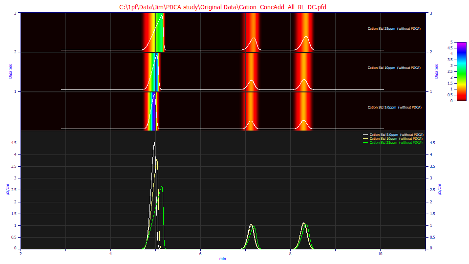
This is a plot of the <e2> genetic algorithm deconvolved data fitted above. Despite the dramatic differences in the peak shapes at the three different concentrations, the fits produce very close to the same overall error, all less than 10 ppm, even with the additional noise introduced by the Fourier deconvolution.
While we assume there is a measure of axial dispersion likely described by the probabilistic half-Gaussian, a measure of mass transfer resistance likely approximated by the 1.5 order kinetic, and we also assume the likelihood of some small first order exponential mixing, this narrow width IRF will probably have to specify just one of these effects. We thus use one of these IRFs for virtually every chromatographic fit:
|
|
Sum of Two First Order Exponentials
|
|
|
Sum of Half-Gaussian and First Order Exponential
|
|
|
Sum of Kinetic Order 1.5 and First Order Exponential
|
The only exceptions have been GC peaks with a slow detector where a single exponential is all that can be fitted and for gradient peaks where a direct fit can be made using a twice-generalized model (adjustments to both third and fourth moments) without an IRF subtraction or fit. In Part III of this white paper series, we will specifically address the unique challenges in fitting gradient HPLC peaks.
 |