GenHVL Extreme Shapes

PeakLab v2 Documentation Contents R2N Software Home R2N Software Support

Concentration Extremes

For certain types of chromatography, extreme concentration shapes can occur where the 64-bit standard floating point (double) precision can no longer mathematically manage the HVL concentration effect. These shapes have been observed in thermal GC separations of polar compounds on non-polar columns with the high-range FID detectors. These high concentration shapes have also been observed in the UHPLC separations that are part of an LC-MS analysis where the mass spectrometer detector is capable of linearly detecting extremely high ionization counts before saturation

These kinds of peaks are seen only when concentrations are very high, the detectors can manage such effectively, and where the column is not going to experience any kind of adsorption site overload. We believe any one of these factors are disqualifying. For example, very high concentrations are typically used with IC preparative chromatography, and the conductivity detectors have all the linearity bandwidth needed, but the ion exchange sites in the column become a limiting factor where column overload shapes rather than high concentration shapes are generally observed.

The GenHVL with 64-bit Floating Point

Before PeakLab v2.00.03, the chromatographic models were capped at a point where the 64-bit precision would overflow the math in the denominator of the HVL-type concentration models:

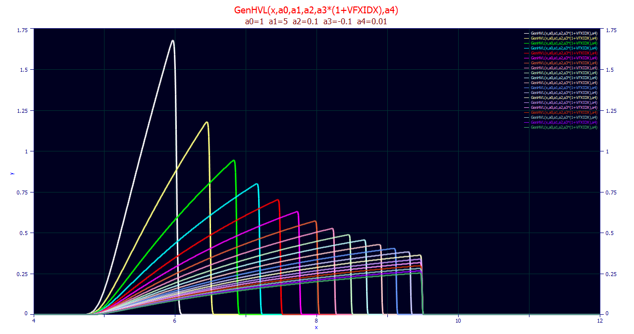
As the a3 concentration dependence term increases, the shapes become more right triangular and elongated. At a certain point, the progression must be capped to accommodate the limitations of 64-bit finite floating point double precision math. Peaks beyond this cap have been experimentally generated, but this has not yet been published.

The GenHVL with 80-bit Floating Point

From PeakLab v2.00.03 onward, when this cap would be imposed, PeakLab switches over to an 80-bit hardware floating point. This was the original precision in the Intel FPUs and it is still available, though far from what is now the norm:

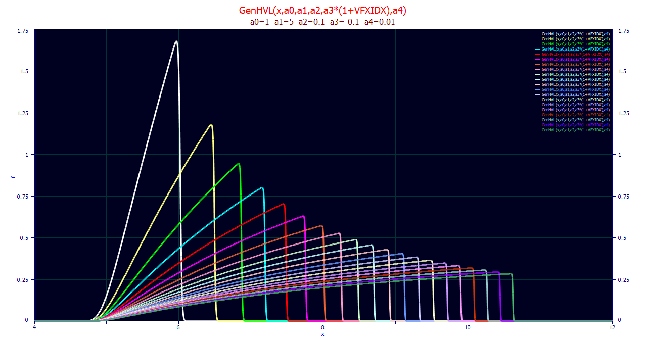
The plot only covers the shape range thus far observed in actual chromatographic runs. The 80-bit floating point processing is capable of even more extreme shapes.

Generalized HVL and Generalized NLC Models

All generalized HVL and NLC models have this automatic 80-bit computational branch for extreme shapes:

GenHVL[Yp2E]
GenHVL[K]

Note that if you are implementing any of these models in your own code, and it is using standard 64-bit math, you will not see the full band of shapes shown in the 80-bit example.

The HVL Model

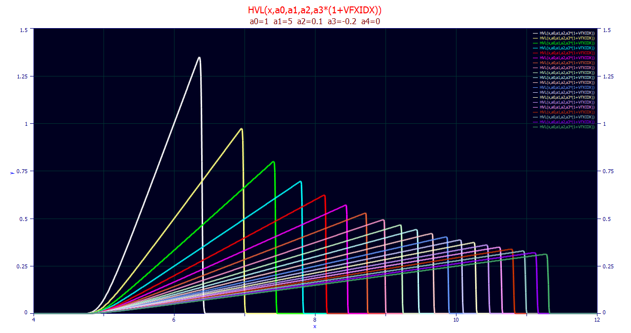
PeakLab's HVL precision-conserving parameterization exploits the symmetry of the Gaussian core density in the HVL so that this 80-bit branch is not needed. The above plot uses 64-bit math for all computations. The concentrations were doubled from the two prior plots.

The NLC Model

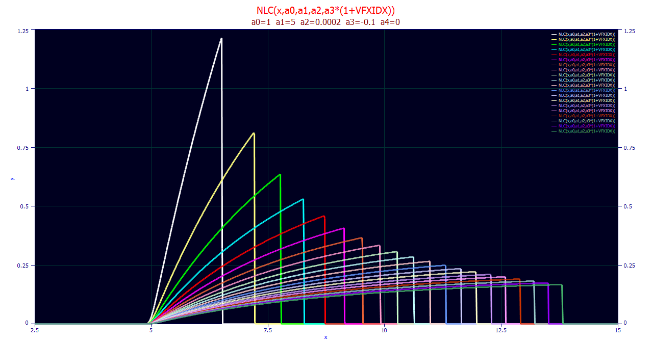
PeakLab's Fast NLC computation uses the generalized normal core density and the NLC distortion's math is essentially identical to the HVL for concentration-dependent distortion. As such, the fast NLC computation (which omits the modified Bessel function and integral), does require the 80-bit processing for extreme shapes. From v2.00.03 onward, the NLC can fit high concentration data to extremely high adsorption rates (very low a2 time constants) as in the tau=12 msec examples above.

Impact of Core Density Third and Fourth Moment on Extreme Shapes

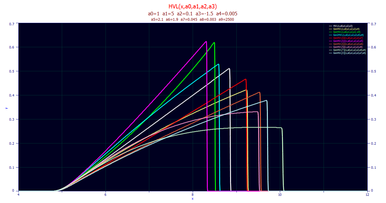
The third and fourth moment parameters of the core density in a generalized HVL model can make a profound difference in peak shape at high concentrations. All of these curves have the same a0 area, the same a1 center location, and the same a2 SD broadening. These a0,a1,a2 parameters can be regarded as representing the zero, first, and second moments. These peaks also share the same a3 concentration dependence, an a3 distortion that would fail with 64-bit precision math.

The white HVL can be seen as the reference point where no specific third or fourth moment adjustments are made to the core density. Note that the HVL exhibits a linear rise.

Add a positive third moment generalized normal skew the core density as is often observed in isocratic separations, and we see the concave yellow GenHVL curve stretched out further in time. Add a negative third moment generalized normal skew to the core density as is often realized in strong gradient separations, and we see the convex green GenHVL curve eluting across a shorter expanse of time. If we instead produce that skewness from a half-Gaussian convolution and adjust its width so that it elutes at approximately the same time as the yellow GenHVL curve, we see the red GenHVL[G] curve above. The GenHVL[G] still appears mostly linear where the yellow GenHVL exhibits an appreciable concave rise.

The picture is even more pronounced with fourth moment compaction and dilation. Add a positive fourth moment error model compaction (power=2.1) as compared to yellow GenHVL (Gaussian power=2.0), as also occurs in strong gradient separations, and we see the cyan Gen2HVL. It actually elutes sooner than the white HVL curve.

If we look at only modifying the fourth moment, and leaving the third moment core density symmetric, we have the magenta and orange GenHVL[Q] peaks. Both the 2.1 and 1.9 parameters for the power of decay produce a linear rise, but there is a huge difference in the peak shapes as a consequence of the fourth moment compaction/dilation. In our experience, gradient separations are about the only way to sharpen this fourth moment.

We will look at a couple of other interesting variations. The pink GenHVL[S] is the Student's t density. It is also symmetric, like the error model used in the GenHVL[Q]. Statisticians generally assume that a nu (degree of freedom) of 100 with a Student's t produces a peak indistinguishable from a Gaussian. If that were true, the pink GenHVL[S] in the plot above, with nu=2,500, would exactly match the white HVL peak. It does not. Mathematically, only a nu ~ infinity would match the HVL.

The GenHVL[T] is a generalized Student's t which, like the generalized error density of the Gen2HVL offers both third and fourth moment parametric adjustments. Adding a small skew to the GenHVL[S], the pink curve, produces the light green GenHVL[T] curve, wider and shifted even further in time. For real-world chromatographic models. a little bit of the far wider Lorentzian tailing (a Student's t essentially varies from a Lorentzian with nu=1 to Gaussian with nu=infinity), goes a very long way. In PeakLab, the nu parameter is directly fitted numerically. You should expect fairly large values of nu if you use these models. It is worth noting that there are Lorentzian models all over the chromatographic literature, but they are purely empirical and there is nothing in fluid dynamics to support a Lorentzian peak shape, unlike spectroscopy where the Lorentzian is the principal theoretical line broadening.

That leaves only the light blue GenHVL[V] curve. This is the only model in PeakLab that offers two different parameters for the third moment asymmetry. It is a combination of the GenHVL[G] half-Gaussian convolution skewness and the GenHVL logarithmic skewness. By varying the amount of each of each different contributions to skewness, you can fit almost any measure of concavity in the rise of a high concentration peak.