PeakLab v2 Documentation Contents            R2N Software Home            R2N Software Support

Extract, Consolidate, and Fit High Resolution LC-MS MS1 Data (Quantitative)

This is the MassSpec | Extract and Fit Quantitative HRMS XICs (IRD)... option. You must first import MS data using the MassSpec | Import MZML data... or the MassSpec | Import Agilent data.ms Data... option.

This option produces the same kind of PeakLab fit as seen with the nonlinear fitting, except the mass spectroscopy information is used to separate the peaks for individual fitting of the consolidated strands. Those are then reassembled into a final PeakLab plot which will contain the molecular peaks, their areas, and their neutral masses.

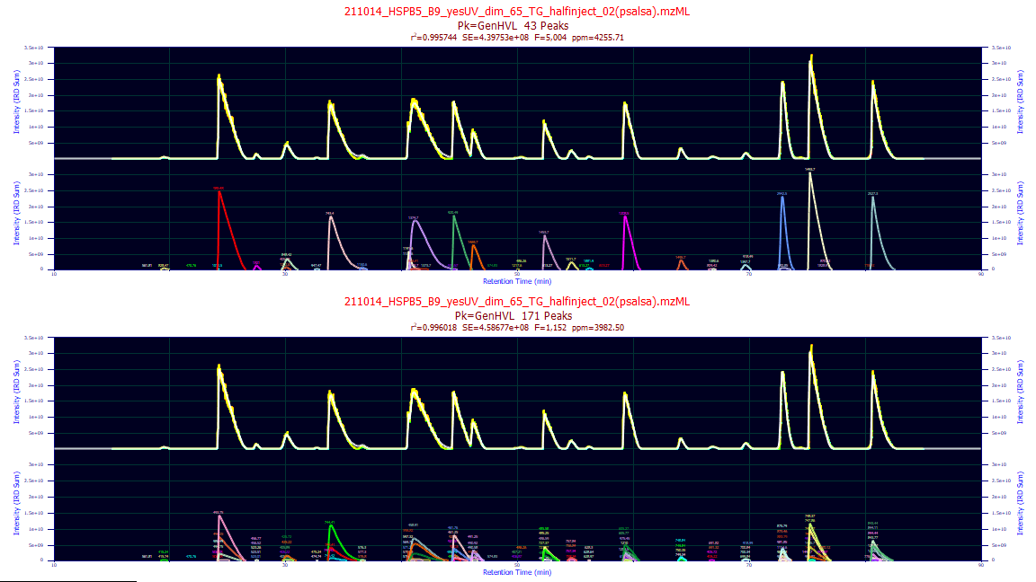
If only a single data set is specified and Omit Raw is not checked, there will be two plots generated. The lower plot will show the fits of each of the unconsolidated strands and the reference data will consist of the sum of the unconsolidated strands (not the TIC). This does mean the signal excluded from the analysis will be absent, which in general means a certain amount of noise filtration occurs. The upper plot will show the fits of each of the consolidated strands and the reference data will consist of the sum of the consolidated strands (again, not the TIC).

Once this procedure has added a mass-spec specific fit to the PeakLab fits, you can optionally refit the consolidated mass spec peaks using PeakLab's nonlinear fitting. In this case, the estimated HRMS peaks are used as the starting estimates for the nonlinear modeling. Whereas coeluting peaks are generally very difficult to process in a nonlinear fit, if the mass-spec peaks are accurate, all should remain very close to their current positions and a small refinement should be seen.

 

If Omit Raw is checked for a single data set fit, or if multiple sets are fit, the unconsolidated plot will not be generated. You will see only a single plot of the aggregated molecules.

To see these fits simply select the MS1 GenHVL or similar entry in the dropdown after the fitting is complete.

Iterative Residual Depletion Algorithm (IRD)

For quantitative analysis of the molecules separated by the chromatography, the Iterative Residual Depletion algorithm represents a fundamental shift in processing high-resolution Liquid Chromatography-Mass Spectrometry (LC-MS) data. Rather than relying on traditional methods, this engine utilizes advanced Digital Signal Processing (DSP) and topology mapping to mathematically extract, group, and deconvolve complex isotopic envelopes, charge states, and co-eluting isomers.

This guide details the underlying algorithms and provides expert guidance on configuring the extraction parameters for optimal PeakLab fitting.

The Algorithmic Pipeline

Data Set Selection

You must first import the HRMS data from MZML files. Use the File menu's Mass Spec Data | Import MZML Data... to load these files into program. At this point you can save out MS1 only MZML files (these are usually much smaller) using the File menu's Mass Spec Data | Save Current Mass Spec Data to MZML Files... or you can use a DSP procedure to filter the background with the File menu's Mass Spec Data | Filter Background/Spikes in MS Data... option. This background filtration algorithm will also save MS1-only MZML files to disk with the background removed from each. Once MZML data have been imported, this MZML fitting option will be available.

Dynamic Ion Trace Detection (IRD)

The analysis begins by identifying the most intense, unassigned mass in the continuous dataset to use as a seed. Instead of projecting a static mass window across the entire retention time, the IRD algorithm dynamically tracks the signal forward and backward in time. By adjusting its search window scan-by-scan based on the local mass apex, it can perfectly trace molecules even when their mass signatures experience parts-per-million (ppm) drift due to space-charge effects or Orbitrap calibration instability.

Charge State & Isotope Consolidation (DBSCAN)

Raw extraction yields thousands of individual isotopic strands. PeakLab utilizes a density-based spatial clustering algorithm (DBSCAN) to group these strands into biologically relevant molecules. By evaluating the Pearson shape correlation (r), temporal apex alignment, and accurate mass differences (accounting for averagine isotopic distributions and common adducts), the engine collapses complex charge-state envelopes into single, quantified neutral mass entities.

The Unified Digital Slicer (Chromatographic Deconvolution)

Co-eluting isomers and unresolved aggregates present massive, asymmetric peak shapes. The Digital Slicer applies a Savitzky-Golay topology map to the consolidated molecule's chromatogram. By analyzing the first and second derivatives, it identifies hidden inflection points and splits multiplexed features into independent chromatographic peaks prior to PeakLab fitting.
 

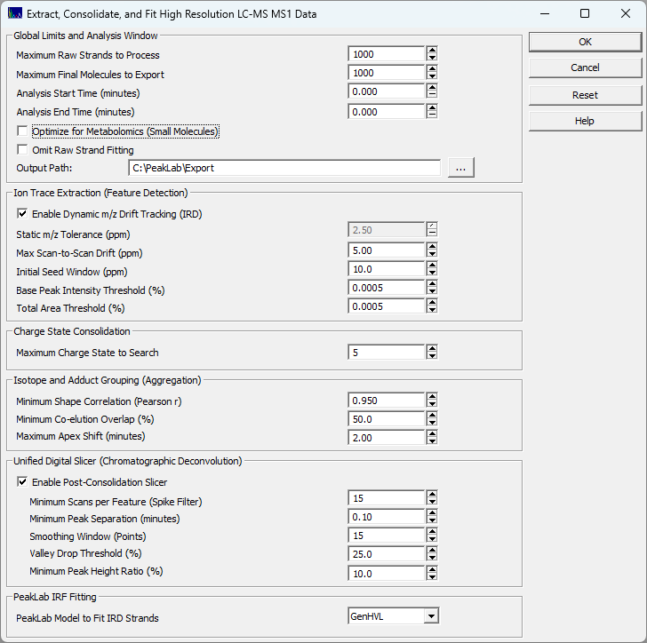
Global Limits and Analysis Window

These parameters dictate the scope and memory footprint of your analysis.

Maximum Raw Strands / Final Molecules

Caps the number of entities processed to prevent memory exhaustion on immensely complex samples. The engine always processes the most intense features first. Warning: setting this too low on highly multiplexed total ion chromatograms (TICs) may truncate low-abundance compounds.

Analysis Start / End Time

Restricts the anaysis to a specific retention time window. Set both to 0.000 to process the entire time range in the separation.

Optimize for Metabolomics (Small Molecules)

This option fundamentally shifts the IRD engine’s chemical logic from a proteomics-based biological model to a generalized, small-molecule physics model.

By default, high-resolution mass spectrometry algorithms are heavily biased toward proteomics (peptides and proteins). Peptides share a highly predictable elemental makeup (Carbon, Hydrogen, Nitrogen, Oxygen, and Sulfur) and readily accept multiple protons during electrospray ionization. Small molecules, lipids, and metabolites, however, are structurally chaotic and require different extraction mathematics.

When you check this box, the IRD algorithm engages two "Smart Overrides" to accommodate small molecules:

Charge State Clamping: Metabolites and small molecules typically carry a single charge (+1) or occasionally +2, unlike large peptides that easily take on +3 to +5 states. When checked, the engine silently overrides your Maximum Charge State to Search setting and strictly clamps it to a maximum of 2. This prevents the algorithm from wasting processing power hunting for impossible charge states.

The Averagine Bypass: Standard proteomics algorithms validate isotopic clusters by comparing them against the Averagine model—a theoretical peak-height probability distribution based on standard amino acids. Metabolites, however, often contain halogens (like Chlorine or Bromine with massive M+2 isotopes), unique elemental ratios, or form salt adducts (+Na, +K) that instantly fail an Averagine test. Checking this box bypasses the strict biological shape filter. If the IRD engine finds signals spaced perfectly by one neutron, it trusts the pure physics and groups them into a molecule, regardless of whether the peak heights match a textbook peptide.

Check this box if you are analyzing metabolites, lipids, sugars, synthetic small molecules, or heavily halogenated compounds. Leave this unchecked if you are analyzing intact proteins, digested peptides, or oligonucleotides.

Important Note on Peak Counts: Because this option strictly caps the charge state at 2, running a proteomics dataset with this box checked will cause the algorithm to reject +3 and +4 peptide groupings. Instead of grouping a +4 peptide's isotopes into a single molecule, it will accurately retain them as separate, independent traces. Your total fitted signal (Y-axis area) and ppm error will remain mathematically similar, but your exported peak count may increase as highly-charged envelopes are split into their unconsolidated components if they are not consolidated by chromatographic location and shape.

Omit Raw Strand Fitting

Crucial for batch processing. When checked, the engine extracts raw strands to allow DBSCAN to function, but discards the massive raw data matrices before fitting. This dramatically reduces RAM usage and export times. It is highly recommended to leave this checked unless you are deeply diagnosing a single file's isotopic grouping.

Output Path

If an output path is specified, diagnostic files will be written to this folder, but only if there is just one mass spec data set being processed. See below for examples of the diagnostic plots written.

Ion Trace Extraction (Feature Detection)

These settings control the sensitivity of the initial mass extraction.

Enable Dynamic m/z Drift Tracking

When enabled, the extraction window shifts scan-by-scan to follow the true mass apex. When disabled, the engine uses the Static m/z Tolerance. Tracking is highly recommended for long gradients or highly concentrated samples where Orbitrap mass drift is common.

Dynamic Step / Drift Catch (ppm)

Max Scan-to-Scan Drift dictates how far the mass apex is allowed to shift between two adjacent scans. Initial Seed Window defines the broad catch-area used to locate the starting point of the trace. Expert Tip: Keep the step tight (e.g., 5.0 ppm) to prevent tracing into adjacent noise, but leave the catch window broader (e.g., 10.0 ppm) to ensure the peak apex is successfully seeded.

Base Peak & Total Area Thresholds (%)

The primary noise filters. These values are percentages of the global maximum intensity (Base Peak) and total TIC area. Values of 0.0005% are typical for deep Orbitrap analysis. Warning: Setting this to 0.0 will cause the engine to extract thousands of pure noise strands, drastically increasing processing time.

Consolidation & Aggregation

These settings govern how individual isotopes are combined into single molecules.

Maximum Charge State to Search

This sets the upper bound of the charge states to process for aggregation. The default number of charge states is 5.

Minimum Shape Correlation (Pearson r)

This is the most important grouping metric. True isotopes of the same molecule will co-elute with nearly identical peak shapes. A value of 0.950 ensures strict chemical fidelity. Lowering this value will force the grouping of noisier, low-abundance isotopes but risks falsely merging different compounds.

Minimum Co-elution Overlap / Max Apex Shift

Requires that isotopic strands physically overlap in time (e.g., 50%) and share a temporal apex within a tight window (e.g., 2.00 minutes or less). This prevents the accidental merging of identical masses that elute at different times in the gradient.

Unified Digital Slicer

For most mass-spec strands, a single peak will be extracted at a given m/z value. The exception are isomers with exactly the same neutral mass which will often appear as discrete peaks in the MS1 XIC. There will be also be aggregations which occurred because the settings allowed two very close m/z strands to be aggregated. Tuning the Slicer is critical for handling these consolidated extracts.

Enable Post-Consolidation Slicer

Activates the topological deconvolution. If disabled, PeakLab will attempt to fit massive, multi-modal blobs, if any, as single peaks, which will likely fail or result in poor statistical fits.

Smoothing Window (Points)

The half-window size for the Savitzky-Golay filter. A value of 15 (resulting in a 31-point moving window) is standard for high-resolution MS. Gotcha: If your data is highly undersampled (very few scans across a peak), reduce this to 5 or 7 to prevent the slicer from obliterating true chromatographic resolution.

Valley Drop Threshold / Min Peak Height

Dictates when a shoulder or convolution is treated as a distinct peak. The Valley Drop (e.g., 25%) requires a distinct dip between two maxima before slicing. The Min Peak Height (e.g., 10%) prevents the slicer from cutting off low-level tailing noise and treating it as a new compound.

PeakLab IRF Fitting

PeakLab Model to Fit

Selects the non-linear mathematical model used to fit the deconvolved data. GenHVL (Generalized Haarhoff-Van der Linde) is the gold standard for chromatography, natively handling the fronting and tailing characteristic of concentration-impacted LC peaks. If the chromatography consists of a mobile phase gradient separation, the twice generalized HVL, the Gen2HVL will allow the 4th moment compaction from the gradient to also be modeled.

Diagnostic Plots

If an Output Path is specified, four diagnostic plots and one Excel-compatible CSV file will be written to that folder. These will only be written for a single data set analysis. They are not written when multiple data sets are selected at the start of this procedure. These will be high resolution 4K PNG graph files that will be overwritten with each single data set run where the Output Path is specified. If you want to preserve these plots, you must save them with a different name before running a new analysis.

peaklab_1_raw_strands.png

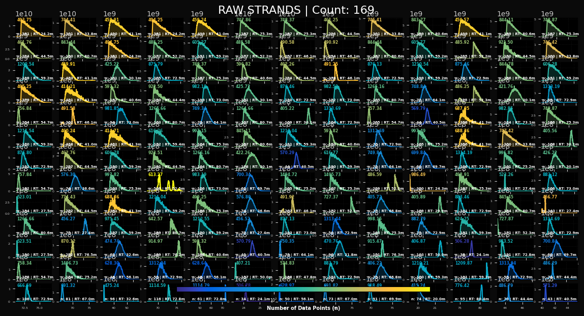
This will plot a matrix of the raw (unconsolidated) IRD strands extracted from the data. Each trace will show the m/z, the n (count of points in the strand), and the RT, the retention time. If you see multiple peaks in a given strand, these could be isomers or a misaggregation. You will probably see some instances especially in the blue low-n strands where the m/z peak was incompletely sampled by the instrument. These often show up as long interpolated linear connections between two widely separated points in time. This file will not be generated if Omit Raw was checked.

peaklab_2_final_molecules.png

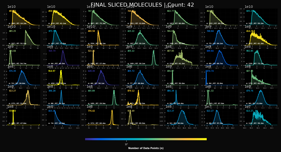
This is the plot of the consolidated molecules. There should be a single peak for each molecule. These are the peaks that will be fit by this procedure. The GenHVL can manage from symmetric peaks to the right triangular high concentration peaks. You may also see a considerable measure of ionization flutter if the analyte concentration was especially high. If you see a peak that is truncated and it is at the upper or lower retention time bound, you should widen the retention time band to accommodate the full peak.

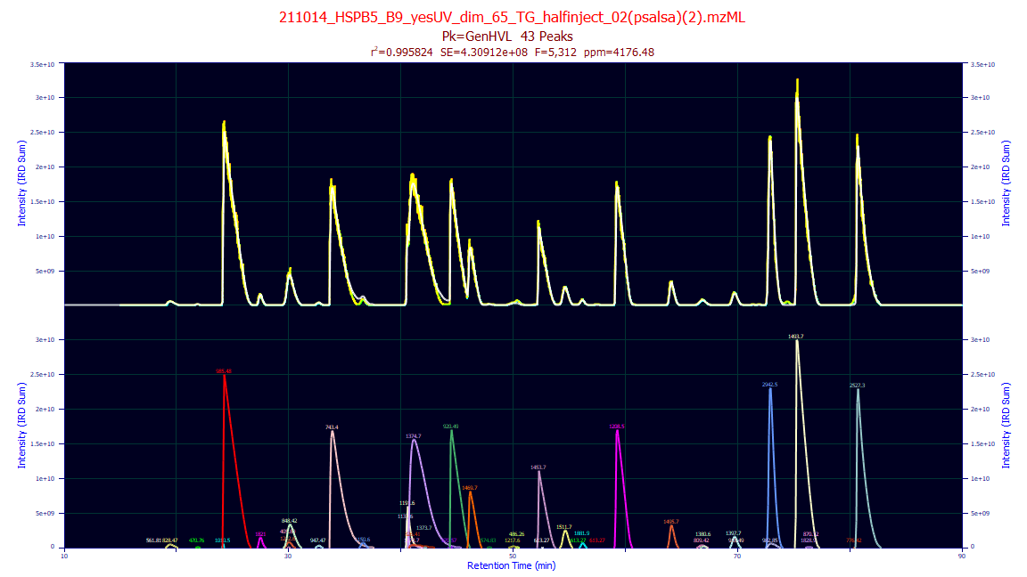
peaklab_3_overlay_linear.png

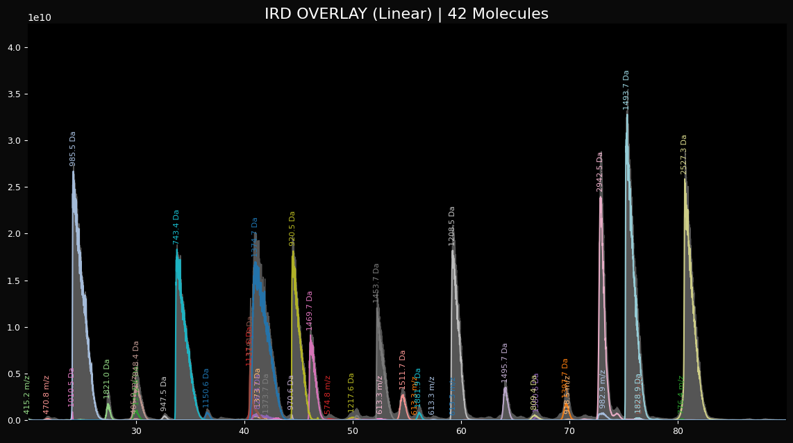
This is a linear plot of the fitted peaks with the estimated neutral masses as the labels.

peaklab_4_overlay_log.png

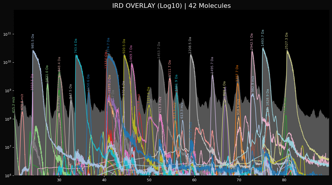
This is a log plot of the peaks that allows you to see what the fitting algorithm had to work with with respect to the noise in the system. Depending on your threshold settings, this plot may show a great deal of noise in the last couple of log decades.

peaklab_final_molecules.csv

 

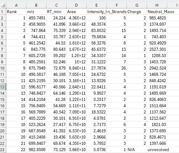
This is a csv file that can be imported into Excel to see the individual summary of the consolidations. If you see an N/A in the charge, and a Neutral_Mass unresolved, this strand was an orphan where there was no information available to compute a charge state. This table will also give you an integrated area of the strands.

A Note on Quantitative IRD Analyses

In PeakLab, quantitative accuracy and "goodness-of-fit" are anchored directly to the raw experimental data. For an analytical algorithm to be considered truly quantitative, the sum of its reconstructed components must approach, but never exceed, the Total Ion Chromatogram (TIC). In the IRD algorithm, the fit statistics are based specifically on the sum of the consolidated or unconsolidated strands—the actual data being fitted—rather than the raw TIC.

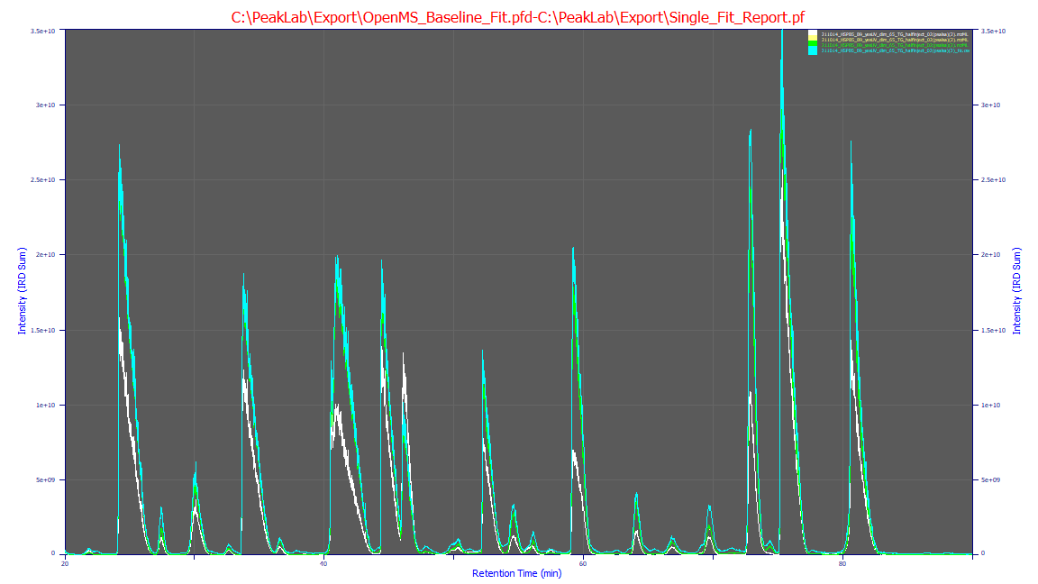
As demonstrated in the plot, the TIC (cyan) serves as the physical upper bound of the measurement. The sum of the IRD strands (green) remains logically just below this bound, representing a faithful, high-fidelity reconstruction of the molecular signal. By definition, a quantitative reconstruction will not perfectly match the TIC, as a small fraction of the background signal and noise is appropriately excluded during the strand extraction process.

For comparison, the OpenMS baseline (white) represents the current industry standard for feature finding using isotopic and charge-state templates. Without the advanced 2D shape-correlation and consolidation logic unique to PeakLab, standard feature finders often fragment broad or overloaded signals into redundant, overlapping features. This leads to the "additive overshoot" visible in the white curve, where the sum of features exceeds the actual raw data.

While OpenMS remains a powerful tool for qualitative feature identification, the IRD algorithm is required for high-fidelity quantitative research where the conservation of mass and signal integrity are of paramount importance.