PeakLab v1 Documentation Contents AIST Software Home AIST Software Support
IRF Model Fits
The Most Effective Chromatographic Instrument Response Functions
For chromatographic peaks which have not been altered in decay by a gradient, where the IRFs are readily fitted, we have three models that have consistently been shown to be superior to all others. These are all two-component models.
The <e2> IRF
This IRF assumes a fast and slow first order kinetic component. For a response function added to the GenHVL and GenNLC models, a4, a5, and a6 are the IRF parameters. In this instance there are two t or time constants fitted for the two exponentials as well as an area fraction of the first component which thus specifies the amount of each component present:
The <ge> IRF
This IRF assumes a half-Gaussian probabilisitic component 'g' and a first order kinetic component 'e'. For analytical, non-preparative shapes, where overload is absent, the exponential is usually the primary or largest width component, and the half-Gaussian will have the smaller width. Again, for a response function added to the GenHVL and GenNLC models, a4, a5, and a6 are the IRF parameters. In this instance there is one t or time constant fitted for the exponential, an SD fitted for the Half-Gaussian, and once more an area fraction of the first (half-Gaussian) component which thus specifies the amount of each component present:
The <pe> IRF
Like the <e2> IRF, this model assumes a fast and slow kinetic component. In this case, there is a first order exponential, the 'e' component, and a 1.5 fractional order kinetic decay, the 'p' component. We again use a4, a5, and a6 for the IRF parameters. In this instance there are two t or time constants fitted for the 'e' exponential and the 'p' 1.5 variable order kinetic decay, and the area fraction of the first component:
The High Width and Low Width Components of an IRF
A two-component model is needed to describe the often usual shape an IRF produces in its tailing
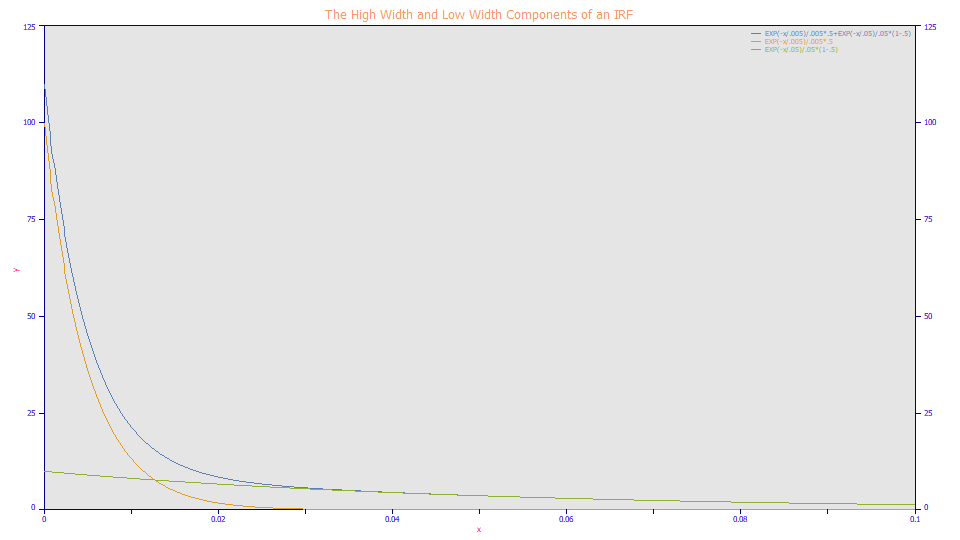
The higher width component will be the predominant determinant of the IRF tailing. The effects of the lower width component will be less even when the fraction of this lower width component predominates.

Here we use the default widths PeakLab uses for the <e2> IRF. We plot the two component IRF and the each of the individual components separately. The fast component governs the decay in the early portion of the curve, and effectively has no influence after a certain point. The slow exponential effects the shape of the elongated tailing, but not the shape in the fast portion of the decay. The fast amber colored curve and the slow green curve, produce the blue curve, the <e2> IRF. When you look at the IRF-originated tailing within the peak, it is difficult to distinguish the impact of the amber component on the overall peak. Visually, it is mostly the green slow component that is observed
A Study of Fitting the Two Components of an IRF
To gauge whether or not we were seeing a system invariant behavior on each of the two components in a two-component IRF, we fitted a strongly fronted IC peak which was generated at various temperatures, concentrations, and additive levels to see if each could be treated as a constant. The fronted peak allows for an effective IRF determination.

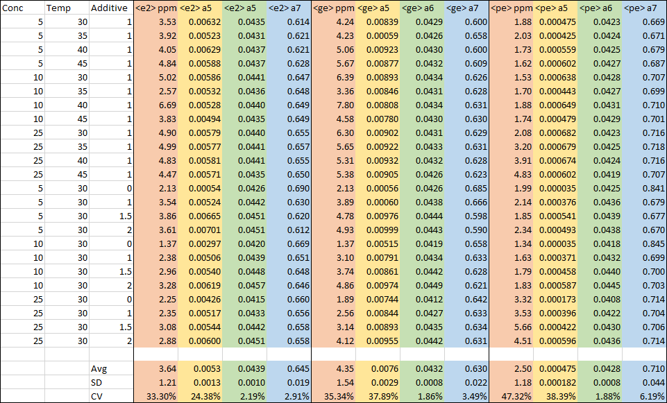
The above table summarizes 24 different data sets, each with three different GenNLC<irf> fits. There are four columns reported for each fit, the ppm goodness of fit and the three IRF parameters. To put these fits in perspective, 3 ppm unaccounted variance is an r2 of 0.999997. Whether we fitting the GenNLC<e2>model, the GenNLC<ge> model, or the GenNLC<pe> model, each of these fits is close to perfect.
The slow or higher width component, always a first order exponential in all three models, is highlighted in green. The values are close to constants irrespective of temperature, concentration, or additive levels. The coefficient of variation is exceptionally small, about 2%. We refer to this component of a two-component IRF as the 'instrument' component, the one that is essentially constant and not impacted by changes in the system variables.
The faster or lower width component is highlighted in yellow. There is a suggestion the GenNLC<pe> model better describes the IRF, but this 1.5 order time constant has a higher coefficient of variation than the first order exponential fast component in the GenNLC<e2>. As you will note this second component is impacted by additive level. The faster or lower width component is not system invariant. We refer to this component of a two-component IRF as the 'system' component, the one that varies with system variables.
The area fraction of the first component is highlighted in blue, and is equally important. Here the variation in the fraction is quite high for the <pe> IRF. This fraction is a measure of the amount of system-varying IRF. In our experience, the fraction will fit to a value where the 'instrumental' or system invariant portion of the IRF is smaller in overall area but of a much higher width (slower rate), and as such the slow exponential will largely influence the overall IRF tailing.
We like the <ge> IRF. In fitting the <ge> IRF, you fit both the simplest probabilistic component and the simplest kinetic component, and at least with respect to axial dispersion there is a validity to the half-Gaussian. In fairness, there is an equal validity to the higher order mass transfer kinetics associated with the migration through porous media, and the <pe> model may manage such, but it is also possible that the second first order exponential in the <e2> represents a good compromise.
We share these results only to illustrate an approach you may wish to use for ascertaining which IRF is most appropriate for your fits. In all likelihood, it will be one of these three primary IRF models.