PeakLab v1 Documentation Contents AIST Software Home AIST Software Support
IRF Estimation - GC
In the LC Estimation examples for the IRF, we focused upon the <ge> and <e2> IRFs, the instrument response functions containing two components, either a sum of kinetic and probabilisitic components, or a sum of two kinetic components. In GC, where it is assumed any kinetics in the chromatography would be too fast to measure, and all can be viewed as a matter of diffusion, you might expect to see very different IRFs. In our experience, the IRFs applicable to LC are also perfectly applicable to GC, even if different mechanisms must be proposed for the components of the IRF.
Fitting a GC Data IRF using the GenHVL<e> Model
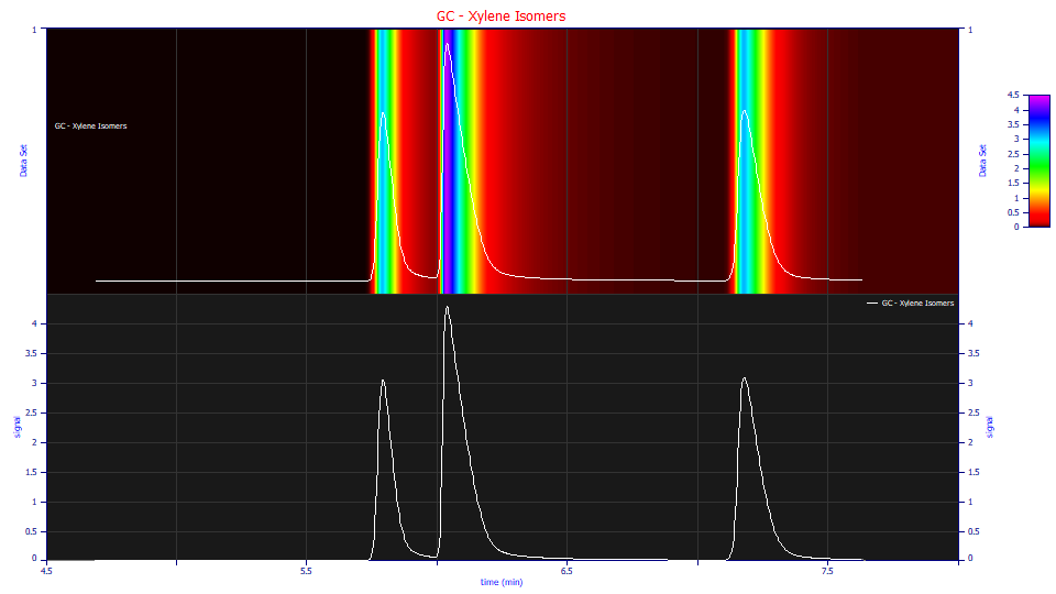
Here we will use GC data where xylene isomers are separated:

The peaks have an elongated tail which is especially apparent in the contour plot in the View and Compare Data option. Such a tail might well suggest a first order exponential IRF is all that is needed to model the decay.
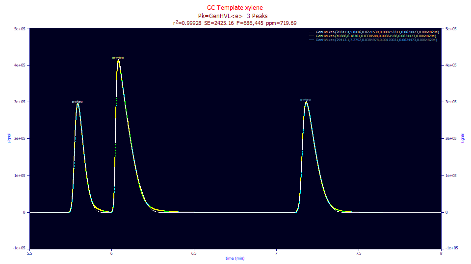
The GenHVL<e> fit to this data has a 719 ppm unaccounted variance, and as is apparent in the plot above, fails to model the instrumental tailing. Here we require the exponential time constant to be shared across all peaks, as is typically done with an IRF. When a peak looks reasonably compact in its decay until near the baseline where it explodes into a major elongation, a two-component IRF is typically needed. A simple exponential cannot convolve a peak and produce this rapidly changing shape. An IRF with both a fast and slow kinetic component, or one with a slow kinetic component and a narrow probabilisitic width, is needed.
Fitting a GC Data IRF using the GenHVL<ge> Model
If we fit the GenHVL<ge> model:

FittedĀParameters
r2ĀCoefĀDetĀĀ DFĀAdjĀr2ĀĀĀĀ FitĀStdĀErrĀĀ F-valueĀĀĀĀĀĀ ppmĀuVar
0.99994693ĀĀĀ 0.99994680ĀĀĀ 658.682599ĀĀĀ 8,070,683ĀĀĀĀ 53.0699319
ĀPeakĀĀ TypeĀĀĀĀĀĀĀĀ ĀĀĀĀĀĀa0ĀĀĀĀ ĀĀĀĀĀĀa1ĀĀĀĀ ĀĀĀĀĀĀa2ĀĀĀĀ ĀĀĀĀĀĀa3ĀĀĀĀ ĀĀĀĀĀĀa4ĀĀĀĀ ĀĀĀĀĀĀa5ĀĀĀĀ ĀĀĀĀĀĀa6ĀĀĀĀ ĀĀĀĀĀĀa7ĀĀĀĀ
ĀĀĀĀ1ĀĀ GenHVL<ge>ĀĀ 21236.2296ĀĀ 5.83193890ĀĀ 0.02504268ĀĀ 0.00053549ĀĀ 0.04171136ĀĀ 0.00599884ĀĀ 0.07673679ĀĀ 0.84599446ĀĀ
ĀĀĀĀ2ĀĀ GenHVL<ge>ĀĀ 40744.2218ĀĀ 6.16032299ĀĀ 0.02910401ĀĀ 0.00240655ĀĀ 0.04171136ĀĀ 0.00599884ĀĀ 0.07673679ĀĀ 0.84599446ĀĀ
ĀĀĀĀ3ĀĀ GenHVL<ge>ĀĀ 30029.3030ĀĀ 7.25943564ĀĀ 0.03435175ĀĀ 0.00121729ĀĀ 0.04171136ĀĀ 0.00599884ĀĀ 0.07673679ĀĀ 0.84599446ĀĀ
The fit is visually much improved and the 53 ppm is close to two orders of magnitude better in the unaccounted variance and all parameters test as significant. It is interesting that 85% of the IRF's area fits to this very narrow half-Gaussian. Only 15% fits to the exponential, and yet this component is responsible for the visible tailing. The IRF deconvolution is shown in the lower plot in red. The very strong tailing of the IRF is removed in this deconvolution.
Fitting a GC Data IRF using the GenHVL<e2> Model
If we fit the GenHVL<e2> model:

FittedĀParameters
r2ĀCoefĀDetĀĀ DFĀAdjĀr2ĀĀĀĀ FitĀStdĀErrĀĀ F-valueĀĀĀĀĀĀ ppmĀuVar
0.99995490ĀĀĀ 0.99995479ĀĀĀ 607.200240ĀĀĀ 9,497,346ĀĀĀĀ 45.0982841
ĀPeakĀĀ TypeĀĀĀĀĀĀĀĀ ĀĀĀĀĀĀa0ĀĀĀĀ ĀĀĀĀĀĀa1ĀĀĀĀ ĀĀĀĀĀĀa2ĀĀĀĀ ĀĀĀĀĀĀa3ĀĀĀĀ ĀĀĀĀĀĀa4ĀĀĀĀ ĀĀĀĀĀĀa5ĀĀĀĀ ĀĀĀĀĀĀa6ĀĀĀĀ ĀĀĀĀĀĀa7ĀĀĀĀ
ĀĀĀĀ1ĀĀ GenHVL<e2>ĀĀ 21227.9396ĀĀ 5.83302708ĀĀ 0.02507899ĀĀ 0.00054290ĀĀ 0.04311635ĀĀ 0.00421864ĀĀ 0.07969028ĀĀ 0.85441528ĀĀ
ĀĀĀĀ2ĀĀ GenHVL<e2>ĀĀ 40752.4698ĀĀ 6.16190676ĀĀ 0.02921077ĀĀ 0.00245103ĀĀ 0.04311635ĀĀ 0.00421864ĀĀ 0.07969028ĀĀ 0.85441528ĀĀ
ĀĀĀĀ3ĀĀ GenHVL<e2>ĀĀ 30043.1433ĀĀ 7.26076525ĀĀ 0.03448250ĀĀ 0.00123519ĀĀ 0.04311635ĀĀ 0.00421864ĀĀ 0.07969028ĀĀ 0.85441528ĀĀ
In the GenHVL<e2>, the the a6 fits to the slow (higher time constant) exponential component with almost the same value and the same area fraction as seen in the GenHVL<ge> fit. The goodness of fit is also somewhat better at 45 ppm unaccounted variance. The better fit coupled with the significance in all parameters, suggests that the <e2> model, the sum of two first-order kinetic delays, is the slightly better IRF model for this GC data set.
The fast exponential component, a5, is about 20x faster, and statistically significant even at this high kinetic rate. This fast component fits to 85% of the overall distortion, but its impact upon the observed tailed shape is small because of this very small time constant.
If the directional Gaussian or probabilistic component of the <ge> IRF mostly addresses the axial dispersion in liquid systems, then it may make sense the two component kinetic model better describes the IRF of GC systems. Here we can only suggest that the GenHVL<e2> may be the model of choice for GC data as opposed to the GenHVL<ge> model. In our development work, we did not have access to GC data with the same exceptional S/N we had in our LC data.
We note that the a4 ZDD asymmetry is high. The program's default, for LC data, is 0.016. These peaks fit to a statistical asymmetry that is almost 3x higher. The a3 chromatographic distortion is also strongly tailed, but did not fit to an increasing trend as the three peaks eluted, unlike the a2 deconvolved Gaussian width which has a clear widening. In this instance, the a3 lack of clear trend may be baseline related. Peaks can appear to be baseline-resolved, as the first two in this data, but the long sloping decay of the IRF may mean there is no decay to an actual baseline between the peaks. If one is actually assigned, errors in the a3 chromatographic shape can occur.
Despite the IRF and intrinsic chromatographic distortion both being tailed, these fits were significant in all parameters and the IRFs were successfully estimated for both models. The narrow width component is somewhat narrower than our LC examples, the wider exponential somewhat larger, and there is more of the narrow component in the overall area, but overall the IRFs are of the same general values. Consider the LC <ge> IRF of the first IRF Estimation example: [0.0080, 0.0432, 0.621]. Here we have [0.0060, 0.0767, 0.846].
We also note that the <e2> and <ge> IRFs are extremely general two-component models. One is a two-component sum of first order kinetic delays and the other a blend of first order kinetic and one-sided probabilistic delays. These are far and away the simplest IRF models that can address such shapes.
Fitting a GC Data IRF using the GenHVL<pe> Model
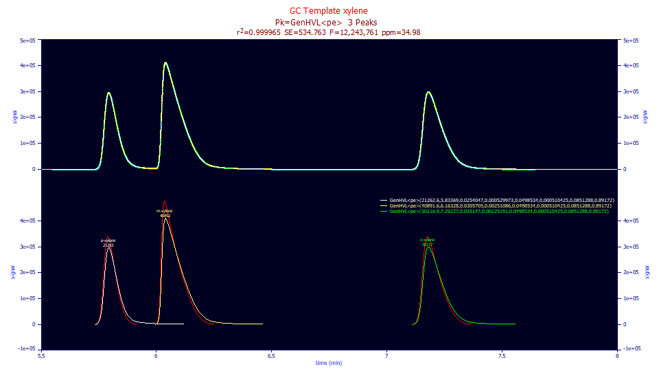
Although we cannot offer an explanation as to why the blend of an order 1.0 and order 1.5 kinetic decay would better fit this data (as in postulating a second order step somewhere in the broadening), we do see an improved fit with the GenHVL<pe> model incorporating this IRF:
FittedĀParameters
r2ĀCoefĀDetĀĀ DFĀAdjĀr2ĀĀĀĀ FitĀStdĀErrĀĀ F-valueĀĀĀĀĀĀ ppmĀuVar
0.99996502ĀĀĀ 0.99996493ĀĀĀ 534.762638ĀĀĀ 12,243,761ĀĀĀ 34.9825784
ĀPeakĀĀ TypeĀĀĀĀĀĀĀĀ ĀĀĀĀĀĀa0ĀĀĀĀ ĀĀĀĀĀĀa1ĀĀĀĀ ĀĀĀĀĀĀa2ĀĀĀĀ ĀĀĀĀĀĀa3ĀĀĀĀ ĀĀĀĀĀĀa4ĀĀĀĀ ĀĀĀĀĀĀa5ĀĀĀĀ ĀĀĀĀĀĀa6ĀĀĀĀ ĀĀĀĀĀĀa7ĀĀĀĀ
ĀĀĀĀ1ĀĀ GenHVL<pe>ĀĀ 21262.5789ĀĀ 5.83369208ĀĀ 0.02540475ĀĀ 0.00052997ĀĀ 0.04985337ĀĀ 0.00051042ĀĀ 0.08512876ĀĀ 0.89172026ĀĀ
ĀĀĀĀ2ĀĀ GenHVL<pe>ĀĀ 40891.5864ĀĀ 6.16327616ĀĀ 0.03057046ĀĀ 0.00251086ĀĀ 0.04985337ĀĀ 0.00051042ĀĀ 0.08512876ĀĀ 0.89172026ĀĀ
ĀĀĀĀ3ĀĀ GenHVL<pe>ĀĀ 30116.9165ĀĀ 7.26226886ĀĀ 0.03514699ĀĀ 0.00125191ĀĀ 0.04985337ĀĀ 0.00051042ĀĀ 0.08512876ĀĀ 0.89172026ĀĀ
The 34 ppm unaccounted variance error is a better goodness of fit and we have an F-statistic of 12.2M as opposed to 8.1M or 9.5M. Here we see an even higher narrow component fraction, perhaps not surprising given that the <pe> IRF's 1.5 order component will have a rapid drop with long sloping tails. All of the parameters fit to significance. This example may be an anomaly, and in general the <pe> IRF is much harder to fit, at least with LC data, but its better fit with this data makes this very different IRF worthy of note.
All three of the two-component IRFs appear to be viable offering exceptional fits with this sample GC data. All produce essentially the same deconvolved a0-a3 HVL values. Even the a4 ZDD asymmetry values are respectably close, a lovely outcome given that the tailed IRF components must coexist with this ZDD asymmetry which is also tailed and which operates on the a3 primary shape which is likewise tailed.
If you find your GC data consistently fits to any one of these three two-component IRF models with 10 ppm error or less, we would greatly appreciate your sharing your experience and sample data with us.
Fitting a GC Data IRF using the GenNLC<pe> Kinetic Model
In all of the prior examples, we used the GenHVL models which fit a diffusion width. Because of how PeakLab implements the GenNLC, it is possible to fit kinetic models. We would expect the kinetic rates to be very, very fast, the time constants exceptionally small, much smaller than the sampling increment of the data:

FittedĀParameters
r2ĀCoefĀDetĀĀ DFĀAdjĀr2ĀĀĀĀ FitĀStdĀErrĀĀ F-valueĀĀĀĀĀĀ ppmĀuVar
0.99996626ĀĀĀ 0.99996618ĀĀĀ 525.168670ĀĀĀ 12,695,210ĀĀĀ 33.7386205
ĀPeakĀĀ TypeĀĀĀĀĀĀĀĀ ĀĀĀĀĀĀa0ĀĀĀĀ ĀĀĀĀĀĀa1ĀĀĀĀ ĀĀĀĀĀĀa2ĀĀĀĀ ĀĀĀĀĀĀa3ĀĀĀĀ ĀĀĀĀĀĀa4ĀĀĀĀ ĀĀĀĀĀĀa5ĀĀĀĀ ĀĀĀĀĀĀa6ĀĀĀĀ ĀĀĀĀĀĀa7ĀĀĀĀ
ĀĀĀĀ1ĀĀ GenNLC<pe>ĀĀ 21252.8995ĀĀ 5.83373093ĀĀ 5.3799e-5ĀĀĀ 0.00052496ĀĀ 10.1960469ĀĀ 0.00050046ĀĀ 0.08261683ĀĀ 0.88691411ĀĀ
ĀĀĀĀ2ĀĀ GenNLC<pe>ĀĀ 40889.9119ĀĀ 6.16294636ĀĀ 7.6178e-5ĀĀĀ 0.00250844ĀĀ 10.1960469ĀĀ 0.00050046ĀĀ 0.08261683ĀĀ 0.88691411ĀĀ
ĀĀĀĀ3ĀĀ GenNLC<pe>ĀĀ 30104.3519ĀĀ 7.26192745ĀĀ 8.437e-5ĀĀĀĀ 0.00124178ĀĀ 10.1960469ĀĀ 0.00050046ĀĀ 0.08261683ĀĀ 0.88691411ĀĀ
Sharing the a4 asymmetry indexed to the Giddings density, the goodness of fit improves slightly. Here we mainly look at a2 and a4 since the other parameters are nearly identical to the GenHVL<pe> which can be deemed a diffusion or statistical peak. As a kinetic peak, we see an a2 first order time constant that increases (the rate slows) with elution location. Its value is 0.000054 to 0.000084 in retention units. As expected, this is much smaller than our sample delta-x of 0.000324. Unlike the arguments in Fourier analysis associated with sampling rate, in fitting a kinetic model we are able to estimate kinetic rates appreciably faster than our sampling.
Even more interesting, perhaps, is the a4 ZDD asymmetry which is indexed to the Giddings first order kinetics at a value of 0.5 (a pure HVL has an a4=0 just as is true with the GenHVL models). With an a4 of 10.2, we fit to an infinite dilution right-skewed asymmetry that is 20x higher than the basic Giddings first order kinetic assumption. These peaks, minus the IRF, are far, far from Gaussian.
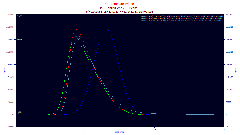
If we look at the different deconvolutions in the Review, the sky blue eluted peak becomes the red peak when the IRF is removed. The removal of the IRF results in a sharpening of the peak and the absence of the long sloping tail. When the red peak's a4 deviation from the HVL is removed, the pure HVL, the green peak, is recovered. It is also a sharply tailed shape. If the green HVL's chromatographic distortion is removed, the pure Gaussian, the bright blue peak, is recovered.
If you compare the sky blue peak as eluted with the bright blue Gaussian, this is a visual indication of just how very far these GC peaks are from Gaussian as registered by the instrument. If you compare the red peak, the eluted peak without the IRF tailing and bright blue Gaussian, the difference is similar. In this instance, the a3 chromatographic distortion is far and away the greatest factor in the non-Gaussian nature of the peak. If you look closely at the deconvolutions it is hard to estimate whether the ZDD non-ideality (represented in the shift between the red and green peaks) or the IRF (the shift between the sky blue and red peaks) is next in terms of impact; only that both are significant.
To fit GC data accurately, you will need to address the IRF, the ZDD non-ideality, and the intrinsic chromatographic distortion just as is done with isocratic LC peaks. GC peaks do not present a simpler fitting problem. In this example, the fit is more demanding: the IRF has greater tailing, the ZDD has a greater deviation from the theoretical zero-distortion shapes, and the a3 chromatographic tailing is appreciable.
Fitting GC Data using the EMG Model
This should suggest the EMG, the model traditionally used for fitting GC peaks, would have a horrible fit. The EMG is the Gauss<e> in our convolution nomenclature, a Gaussian as the core peak, and a single component first order exponential as the IRF:
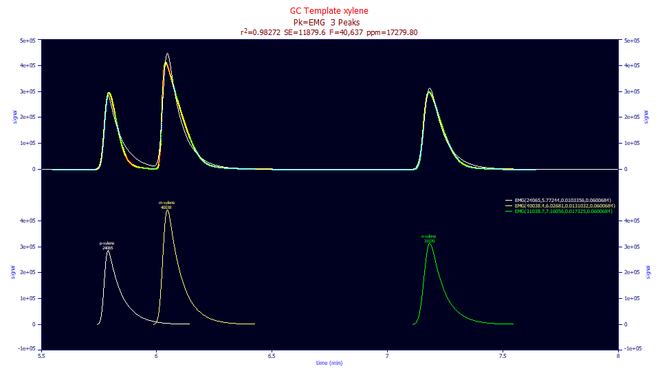
For this data, the EMG fits to 17,280 ppm error when the <e> width is shared across the peaks. These chromatographic peaks, with the system IRFs removed, are strongly non-Gaussian.
The number of models in PeakLab that are capable of reducing to an EMG requires a page's worth of listing. Every model we fit in this topic will reduce to an EMG if the IRF can be reduced to a single component exponential and the core peak to a pure Gaussian. We strongly suggest that you waste no time fitting the EMG separately. If by some chance you actually have an EMG or Gauss<e> peak, these other models will reduce to that shape.
Fitting GC Data using the HVL Model
With no IRF modeling, the HVL fit would also be expected to suffer the error arising from not accommodating the IRF or the nonideality in the ZDD:
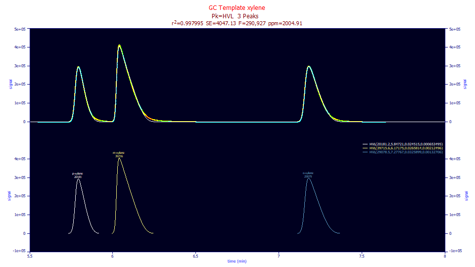
The error in this fit is 2,005 ppm unaccounted variance.
We illustrate the EMG and HVL fits to this data as eluted to illustrate the state of the fitting science as it existed across decades. It is possible that nonlinear modeling of chromatographic peaks never saw the valuation it should have had to a large measure because of that which is shown in these last two fits. For decades, these two models represented the two primary choices offered in nonlinear fitting software. You could have an incomplete IRF with a Gaussian, or an incomplete chromatographic shape with no IRF. Both fits come nowhere near what is realized when accounting both the IRF and ZDD in a complete chromatographic modeling. Contrast these poor EMG and HVL fits with the 30-60 ppm error GenHVL<ge>, GenHVL<e2>, and GenHVL<pe> fits.
Note that the GenHVL and GenNLC models, even with IRFs, will fit to the HVL and NLC shapes if there is no IRF present (something we have never observed) and if there is no ZDD non-ideality (exceptionally rare and probably not real). Further, a generalized HVL will fit both the HVL and NLC shapes. The generalized NLC model will likewise fit both shapes.