PeakLab v1 Documentation Contents AIST Software Home AIST Software Support
IRF Estimation 1 - Standards Containing One or More 'Fronted' Peaks
An IRF determination can be straightforward, even though when you seek to determine an instrument's response function, you will be simultaneously using one of the most sophisticated processes of statistical fitting as well as one of the most demanding procedures in signal processing.
Fronted Peaks
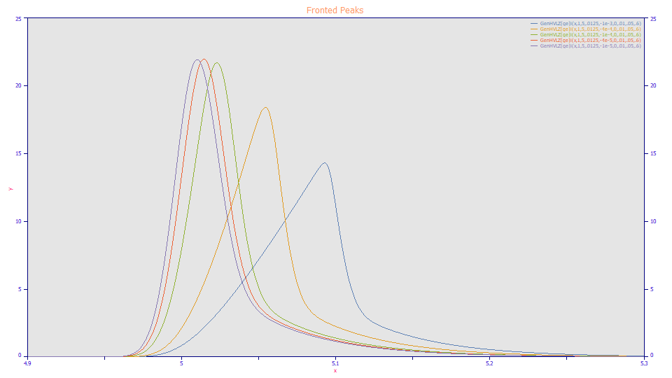
In PeakLab, when we refer to fronted peak, we are specifying a left-skewed peak after the instrument response function (IRF) has been removed. A fronted peak, within PeakLab, is defined as a peak where the chromatographic separation skews more of the mass of the peak to the left of the mode or apex of the peak than to the right. This intrinsic fronted nature may not be apparent after instrumental distortions add their right skew. Instrumental distortions are almost always tailed, adding kinetic delays (usually treated as an aggregate first order exponential) and/or one-sided probabilisitic deviations (usually treated as a half-Gaussian) to the broadening.
After the IRF has been removed by either a preprocessing deconvolution step, or by fitting a <irf> bearing model, a negative third moment (statistical skew) indicates an intrinsically fronted peak, one where the chromatographic separation distributes the mass about the apex such that a greater measure of the mass appears prior to the apex or mode of the peak.
Similarly, after the IRF has been deconvolved, a positive third moment indicates an intrinsically tailed peak, one where where the chromatographic separation distributes the mass in the opposite direction. The greater measure of the mass elutes after the peak apex.
With respect to methods for estimating the instrument response function (IRF) of a chromatographic instrument/system, one or more fronted peaks are usually sufficient to furnish enough independence in the different parameters to produce an accurate estimate of the non-chromatographic distortion or IRF in the peaks. In PeakLab, we generally assume the IRF to be constant across all peaks in a fit, and generally constant for a given instrument, column, prep, and run conditions. As such we add at most three parameters to any given model<irf> fit, these specific IRF parameters shared across all peaks.
The prevailing view in chromatography is that fronted peaks are quite rare. By our practical definition, fronted peaks are actually quite common. They may simply appear to be tailed peaks as a consequence of the instrumental distortion.

In your chromatograms, you may well see peaks such as those above. The first three peaks would be readily classified as 'tailed'. You might call the fourth peak indeterminate, and the only the last peak as possibly 'fronted'. By our definition, all of these peaks are intrinsically fronted and perfect candidates for this first IRF Estimation approach, which is little more than fitting all the peaks in a clean standard to a model containing an <irf>.
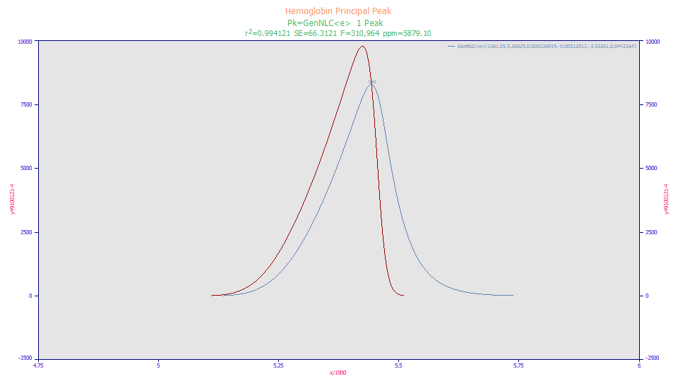
This is the very large peak that occurs in a hemoglobin analysis. Here only this principal peak was fitted, all other peaks ignored, and only to a GenNLC<e>, the generalized NLC with a simple exponential IRF. The peak we address is the IRF deconvolved peak, the red peak in the plot, which is quite clearly fronted when contrasted with the peak the instrument reported. Many peaks are viewed as tailed only because of the instrumental effects or distortions which introduce tailing.
For many early eluting peaks, the deconvolved peak, the 'true' peak that would exist free of the IRF, is fronted with respect to its shape independent of instrumental distortions.
Fitting Data for IRF Estimation
In exploring the different approaches to IRF determination, we will use a standard where one or more of the peaks elute early enough to have this fronted shape. In the following data, we have three different concentration series which span half a year's time. This data is an IC standard which consists of six peaks, three fronted, three tailed. The standards were run at concentration of the solutes varying from 1 ppm to 25 ppm.
A fronted peak will have a left shifted intrinsic chromatographic skew (a negative a3 parameter). An IRF adds tailing as a consequence of unidirectional kinetic and/or probabilisitic effects. If one or more fronted peaks exist, for those peaks there will be two distinct and opposing skews to the peak, the intrinsic chromatographic skew (the left skew specified by a3 and a4 in the GenHVL and GenNLC models), and the IRF skew (the right skew specified by the IRF parameters). The lesser likelihood of correlation between the parameters means that the IRF may be more accurately estimated, so much so the presence of a number of tailed peaks will not harm the estimation.
An IRF should be reasonably independent of the concentration of the solutes for peaks which are fitted. An instrumental response function would ideally smear or distort very low concentration peaks identically to high concentration peaks. This is generally true, but in this example we will wisely seek to confirm this concentration independence using different concentrations of the standard.
In this IRF estimation method where we use standards containing a mix of fronted and tailed peaks, we make no effort to section the data so as to only include the fronted peaks. It is assumed the shared IRF parameters across all peaks will be such that the fronted peaks will constrain the fit, addressing any adverse positive correlation between the tailed peaks and the tailed IRF. This first approach includes such tailed peaks in the IRF estimation.
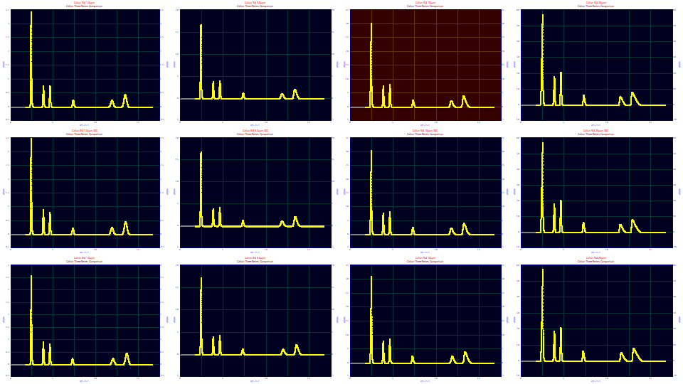
We thus have a matrix of twelve chromatograms, three different runs of the standard at very different times, and for each, four very different concentrations. The first panel in each of the three series, the 1 ppm concentration, will have very little chromatographic distortion. The last panel, 25 ppm, will have strongly fronted and tailed peaks.
Concentrations Used in IRF Estimation
The approach historically used for IRF estimation would be to generate very low concentration Gaussian-like peaks and fit an EMG to the data to ascertain the tau or exponential width or time constant of the delay inherent in the detector which the IRF traditionally estimated.
In PeakLab, you will generally want to do the reverse. You will want to fit data with a considerable chromatographic skew to ensure the higher moments can be fitted and also to avail yourself of a higher S/N. Further, in PeakLab we want to fully map the instrumental distortion. In order to do so, we want to realize near-perfect fits.
We thus begin with the obvious problem that arises when fitting IRFs when the concentrations are so low the peaks have very little a3 chromatographic distortion.
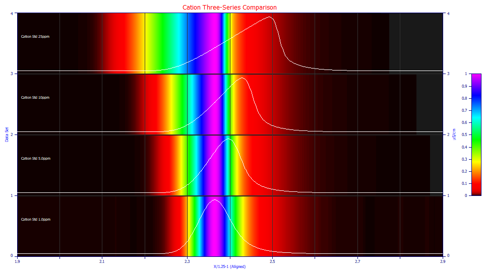
This is the first peak (the most fronted) in the first concentration series using the View and Compare Data option. The 25 ppm concentration is at the top, the 1 ppm concentration at the bottom. If you look closely at the tailing in the unit magnitude aligned contours, or in the actual decay of the tails in the peaks, you can see the IRF in each, and to the eye each appears identical.
If you ignore the tailing and look only at the overall peak shape, the 25 ppm concentration has a strongly fronted shape. It is less in the 10 ppm peak, and lesser still in the 5 ppm peak. The 1 ppm peak has so little chromatographic distortion, it is difficult to know whether to label the peak as fronted or tailed. When a GenHVL or GenNLC model is fitted, the a3 intrinsic chromatographic distortion will be very close to linear with concentration. This means the 25 ppm peak will be 25 times more fronted or distorted than the 1 ppm peak and it will also have a S/N that is 25 times higher.
The problem with fitting the 1 ppm concentration to estimate the IRF isn't the absence of the IRF, for it is present. It isn't even the 25x decrease in S/N, for here the data are still sufficient to model the IRF. The problem lay in the fact there is so little chromatographic distortion, a3 will be close to zero. The a4 asymmetry parameter in the GenHVL and GenNLC models alters the shape of the zero distortion density, but that only factors into the peak shape to the extent of a3. When the intrinsic a3 distortion is too close to zero to accurately estimate at a weak S/N, the a4 can assume almost any value.
There are a host of ways to address the inability to fit the the 1 ppm data with a generalized model, and these have nothing to do with IRF estimation. For example, one can fit the GenNLC with a4 locked at 0.5 in the ZDD configuration (forcing the peak to be a pure NLC), one can fit the NLC directly. The problem with fitting a 1 ppm sample has much more to do with the chromatographic model itself.
In our experience, the best IRF determinations will be made when the chromatographic distortion and S/N is high, the non-idealities in the density well mapped by the a4 in a GenHVL or GenNLC model, and either the <ge> or <e2> IRF is used to model the instrumental distortion.
The <ge> Half-Gaussian, Exponential IRF
The <ge> IRF, is a variable area sum of both a half-Gaussian 'g' probabilisitic distortion, and an exponential 'e' first order distortion. It is the 'go-to' IRF in the program, the one that has consistently fitted every analytic sample we ever estimated for non-gradient LC and GC data. As discussed in the overview of IRF estimation, the <ge> model is the simplest possible model for an IRF where axial dispersion, generally believed to be Gaussian in broadening, occurs.
The <e2> Two-Exponential IRF
The only other IRF we have found to be both highly effective and easy to fit in high precision analytical peak modeling is the <e2> where two different exponential decays are assumed to simultaneously occur. In this case there is a fast and slow exponential component. Although our data are limited, we have seen GC data better fitted with the <e2> IRF. In this first IRF estimation example, we will also estimate an IRF using this <e2> model.
The 1 ppm Fits to the GenNLC<ge> Model
We will begin by simultaneously fitting all twelve data sets to the GenNLC<ge> model in order to estimate the three parameters of the <ge> IRF.
Let's look at one of the 1 ppm fits:
Fitted Parameters
r2 Coef Det DF Adj r2 Fit Std Err F-value ppm uVar
0.99997628 0.99997622 0.00123575 17,325,246 23.7220441
Peak Type a0 a1 a2 a3 a4 a5 a6 a7
1 GenNLC<ge> 0.35216350 2.34936850 0.00025131 -0.0002543 -0.5940143 0.00118785 0.04172193 0.55398517
2 GenNLC<ge> 0.09979369 3.80350522 0.00026496 -4.031e-5 -0.5940143 0.00118785 0.04172193 0.55398517
3 GenNLC<ge> 0.10673861 4.57580601 0.00025676 -6.765e-5 -0.5940143 0.00118785 0.04172193 0.55398517
4 GenNLC<ge> 0.05258585 7.31171927 0.00038608 7.3705e-5 -0.5940143 0.00118785 0.04172193 0.55398517
5 GenNLC<ge> 0.08837613 11.8847692 0.00081331 0.00051216 -0.5940143 0.00118785 0.04172193 0.55398517
6 GenNLC<ge> 0.17915516 13.4733266 0.00083416 0.00144711 -0.5940143 0.00118785 0.04172193 0.55398517
As discussed above, a GenNLC fit is not tenable. The a3 chromatographic distortion is very close to zero, and the a4 asymmetry has assumed an uncharacteristically negative value (it is typically between 1-2, an asymmetry greater than the 0.5 Giddings ZDD of the NLC). Although the grayed values above show the a5 and a7 parameters to have lost significance (which is true), we know why this occurred. The model itself is statistically overspecified.
The 5,10,25 ppm Fits to the GenNLC<ge> Model
The Numeric Summary of the fits offers an Average Multiple Fits option in the Options menu which we use to automatically get the averages of the IRF from the fitted peaks of all of the data sets. The higher concentration fits are excellent, many with less than 10 ppm unaccounted variance.
In PeakLab there is no need to refit just the data sets we wish to use in order to automatically average the IRF. In the Review, select or highlight only the graphs of the fits you wish to average (simply click on them to produce the gray border) and then right click on any graph and select Plot | Only Selected Fits. The Numeric Summary will change to reflect only the selected fits. If we select just the 5, 10, and 25 fits, we see the following average and CV% (coefficient of variation) for the nine fits.
Average for 9 Fits
Fitted Parameters
r2 Coef Det DF Adj r2 Fit Std Err F-value ppm uVar
0.99999201 0.99999199 0.00823536 54,496,137 7.98568653
Peak Type a0 a1 a2 a3 a4 a5 a6 a7
1 GenNLC<ge> 4.71460251 2.31707192 0.00024094 -0.0059171 1.19121998 0.00802842 0.04315663 0.62100260
2 GenNLC<ge> 1.31720395 3.78584950 0.00027810 -0.0009170 1.19121998 0.00802842 0.04315663 0.62100260
3 GenNLC<ge> 1.52788201 4.55993418 0.00026680 -0.0004145 1.19121998 0.00802842 0.04315663 0.62100260
4 GenNLC<ge> 0.69048931 7.26556321 0.00039275 0.00114750 1.19121998 0.00802842 0.04315663 0.62100260
5 GenNLC<ge> 1.17015453 11.9045847 0.00081613 0.00758438 1.19121998 0.00802842 0.04315663 0.62100260
6 GenNLC<ge> 2.39533580 13.5703790 0.00089913 0.01654189 1.19121998 0.00802842 0.04315663 0.62100260
CV Percent for 9 Fits
Fitted Parameters
r2 Coef Det DF Adj r2 Fit Std Err F-value ppm uVar
0.00020604 0.00020655 62.3811419 25.6355593 25.8009445
Peak Type a0 a1 a2 a3 a4 a5 a6 a7
1 GenNLC<ge> 67.4869447 0.88554754 4.33552791 65.9818065 8.48321303 15.2152332 0.86586822 1.74677118
2 GenNLC<ge> 67.4451709 0.22549963 3.30853818 67.3205706 8.48321303 15.2152332 0.86586822 1.74677118
3 GenNLC<ge> 67.5881699 0.15981790 1.32268080 68.4295031 8.48321303 15.2152332 0.86586822 1.74677118
4 GenNLC<ge> 67.4280964 0.43640004 0.70373863 79.0151555 8.48321303 15.2152332 0.86586822 1.74677118
5 GenNLC<ge> 67.5620094 0.52383975 0.63360044 66.7250949 8.48321303 15.2152332 0.86586822 1.74677118
6 GenNLC<ge> 67.5370342 0.64559572 2.72759586 67.0997786 8.48321303 15.2152332 0.86586822 1.74677118
The average <ge> IRF for the 5-25 ppm fits is [0.00802842, 0.04315663, 0.62100260]. Across the concentrations and different samples in time, the coefficient of variation for the 'e' component of the IRF is superb, less than 1%. The ratio is also excellent, a CV of just 1.75% (the CV table consists entirely of % values). It is only the much smaller 'g' width which has the higher CV of 15.2%. In our experience, that is still remarkably good given the differences across concentration and column states. Its lack of absolute constancy with concentration (there is a slight increase with concentration) perhaps lends support to the premise this Gaussian component includes the axial dispersion.
These <ge> parameter values can be input into the IRF option to have these values used as the default starting estimates for the fitting algorithm. The purpose of the IRF and ZDD dialog options in the program is to have this experience reflected in the program's default estimates.
Note that you can also lock these <ge> values in performing fits with this <ge> IRF as an alternative (albeit a much slower one) to using Fourier deconvolution prior to fitting. When fitting an <irf> model, discrete Fourier methods are used in the fitting for the convolution integral. Such will be far faster than directly fitting the integrals, but fits which can take mere seconds with pre-deconvolved data, may require minutes when this Fourier deconvolution must be computed for every point in every peak in every iteration of a fit.
More importantly, when these IRF values are set as the default <ge> IRF values, they are the values offered in the Fourier IRF Deconvolution preprocessing option which is used to preprocess data by removing the instrumental distortions prior to fitting. While we cannot characterize how constant such IRFs are relative to instruments, columns, and preps, we can note that we have observed stable IRFs across columns of a given type, and across variations in temperature, additives, and concentrations. It is also important to note that if these estimated IRF values are not appropriate to a given data set, such will generally be visibly obvious in this Fourier deconvolution preprocessing step.
The 5,10,25 ppm Fits to the GenNLC<e2> Model
The area-weighted sum of two exponentials is the only other IRF we have found to be truly effective in analytical peak modeling which can be consistently fitted. Two different exponentials, a fast and slow decay, are assumed to simultaneously occur. If we perform a similar process with the GenNLC<e2> model we see the following:
Average for 9 Fits
Fitted Parameters
r2 Coef Det DF Adj r2 Fit Std Err F-value ppm uVar
0.99999253 0.99999251 0.00794235 58,851,411 7.47316661
Peak Type a0 a1 a2 a3 a4 a5 a6 a7
1 GenNLC<e2> 4.71537133 2.31812020 0.00024132 -0.0059024 1.23357325 0.00551566 0.04370803 0.63718806
2 GenNLC<e2> 1.31742426 3.78683148 0.00027797 -0.0009185 1.23357325 0.00551566 0.04370803 0.63718806
3 GenNLC<e2> 1.52817753 4.56089398 0.00026672 -0.0004168 1.23357325 0.00551566 0.04370803 0.63718806
4 GenNLC<e2> 0.69052696 7.26633965 0.00039278 0.00113928 1.23357325 0.00551566 0.04370803 0.63718806
5 GenNLC<e2> 1.17017802 11.9052506 0.00081700 0.00757332 1.23357325 0.00551566 0.04370803 0.63718806
6 GenNLC<e2> 2.39544711 13.5711254 0.00090117 0.01654543 1.23357325 0.00551566 0.04370803 0.63718806
CV Percent for 9 Fits
Fitted Parameters
r2 Coef Det DF Adj r2 Fit Std Err F-value ppm uVar
0.00021279 0.00021333 63.2166433 27.4993697 28.4736325
Peak Type a0 a1 a2 a3 a4 a5 a6 a7
1 GenNLC<e2> 67.4898003 0.83840245 4.94668366 65.6204282 8.29774245 4.83522376 0.73131915 2.84687749
2 GenNLC<e2> 67.4488013 0.20301825 3.56597818 66.5981050 8.29774245 4.83522376 0.73131915 2.84687749
3 GenNLC<e2> 67.5913765 0.14590807 1.53677852 67.1922628 8.29774245 4.83522376 0.73131915 2.84687749
4 GenNLC<e2> 67.4424843 0.43471807 0.81652847 79.6907122 8.29774245 4.83522376 0.73131915 2.84687749
5 GenNLC<e2> 67.5641503 0.52250031 0.58940125 66.9247013 8.29774245 4.83522376 0.73131915 2.84687749
6 GenNLC<e2> 67.5373109 0.64737113 2.74259847 67.1878572 8.29774245 4.83522376 0.73131915 2.84687749
Here we see a delightful confirmation of the 0.043 exponential width we saw in the <ge> fit and well as very close to the same area fraction of the higher and lower width components. Here the fast exponential also has a CV (4.8%) that is about a third of the half-Gaussian in the <ge>, although the area fraction defining the amount of the two exponential components has a CV somewhat higher (2.8%).
In our experience the 'e' component of the <ge> model, and the slower exponential with the larger tau in the <e2> model, will be very close to constant across temperatures, additive levels, and concentrations. It is the much faster component in each IRF which will evidence less constancy.
As to whether you use the <ge> or the <e2> IRF, PeakLab offers both in its default chromatographic models. The <ge> may be the more theoretically appropriate in LC, but you may find the <e2> of benefit, and as above, with a slightly better fitting. In all likelihood, the fast component of the IRF is likely to be a mix of multiple probabilistic and kinetic effects.
In PeakLab, user-defined peaks offer an automatic <ge> and <e2> IRF convolution option. These are the only user-defined two-component IRF convolutions made available in the program. In our experience with LC data, there will almost always be both a slow and fast IRF component. At one point we had over 100 different IRFs in the program during the development phase. In the final analysis, no IRFs have performed as well, as consistently, and as stably as the <ge> and <e2> models. In our limited work with GC data, we also consistently observed both a fast and slow component in the <e2> IRF. A single <e> never worked well.
The 5,10,25 ppm Fits to the GenNLC<e> Model IRF - the EMG Legacy
As a matter of interest, here is the similar summary for the GenNLC<e> model where just a single exponential is used for the IRF.
Average for 9 Fits
Fitted Parameters
r2 Coef Det DF Adj r2 Fit Std Err F-value ppm uVar
0.99934961 0.99934809 0.07962334 733,077 650.387303
Peak Type a0 a1 a2 a3 a4 a5
1 GenNLC<e> 4.64601148 2.29656497 0.00015338 -0.0065110 1.82986331 0.02631961
2 GenNLC<e> 1.29897420 3.77811316 0.00026921 -0.0008854 1.82986331 0.02631961
3 GenNLC<e> 1.50965230 4.55440984 0.00026198 -0.0003193 1.82986331 0.02631961
4 GenNLC<e> 0.68866779 7.26339413 0.00039620 0.00133088 1.82986331 0.02631961
5 GenNLC<e> 1.17041881 11.8968009 0.00083145 0.00752298 1.82986331 0.02631961
6 GenNLC<e> 2.39622329 13.5614921 0.00092535 0.01635924 1.82986331 0.02631961
CV Percent for 9 Fits
Fitted Parameters
r2 Coef Det DF Adj r2 Fit Std Err F-value ppm uVar
0.01664255 0.01668157 68.2025287 30.8380103 25.5720349
Peak Type a0 a1 a2 a3 a4 a5
1 GenNLC<e> 67.5091990 0.80908953 4.08057910 66.5358203 60.0757017 8.76917765
2 GenNLC<e> 67.3460346 0.13958063 7.51784255 60.7630293 60.0757017 8.76917765
3 GenNLC<e> 67.4958494 0.13218893 4.50990881 64.5885955 60.0757017 8.76917765
4 GenNLC<e> 67.4932952 0.44829356 1.12841436 80.2092810 60.0757017 8.76917765
5 GenNLC<e> 67.5371174 0.51241404 2.61007034 68.7855596 60.0757017 8.76917765
6 GenNLC<e> 67.4500604 0.65388589 2.12863127 65.9248533 60.0757017 8.76917765
We note that the single exponential <e> IRF is not likely to be of much use in modern-day LC data. In a similar analysis, note the average of 650 ppm unaccounted variance across the nine fits in contrast with the 8 ppm of the <ge> and <e2> IRFs. This higher error was typical of all of the <e> fits, not one very poor fit throwing off the average.
The 5,10,25 ppm Fits to the NLC<ge>
How important is the higher moment information in a generalized model? Here is the similar nine-data set average for the NLC<ge> model where the a4 ZDD asymmetry term in the generalized model is no longer present:
Average for 9 Fits
Fitted Parameters
r2 Coef Det DF Adj r2 Fit Std Err F-value ppm uVar
0.99996716 0.99996708 0.01921813 20,653,210 32.8422191
Peak Type a0 a1 a2 a3 a4 a5 a6
1 NLC<ge> 4.72125605 2.31914610 0.00026255 -0.0031340 0.00557226 0.04347472 0.64465888
2 NLC<ge> 1.31757542 3.78941800 0.00028305 -0.0004296 0.00557226 0.04347472 0.64465888
3 NLC<ge> 1.52811950 4.56347312 0.00026941 -0.0001794 0.00557226 0.04347472 0.64465888
4 NLC<ge> 0.69029414 7.26945370 0.00038952 0.00060462 0.00557226 0.04347472 0.64465888
5 NLC<ge> 1.16892276 11.9088878 0.00079034 0.00376226 0.00557226 0.04347472 0.64465888
6 NLC<ge> 2.39156680 13.5718002 0.00085181 0.00795982 0.00557226 0.04347472 0.64465888
CV Percent for 9 Fits
Fitted Parameters
r2 Coef Det DF Adj r2 Fit Std Err F-value ppm uVar
0.00232453 0.00233019 89.1725231 66.3019870 70.7764988
Peak Type a0 a1 a2 a3 a4 a5 a6
1 NLC<ge> 67.5052175 1.08257058 2.72185298 70.0601101 79.6968375 0.68126561 3.81218567
2 NLC<ge> 67.4538690 0.29169682 3.53095747 73.6297216 79.6968375 0.68126561 3.81218567
3 NLC<ge> 67.5896325 0.19803844 1.26131427 80.2686625 79.6968375 0.68126561 3.81218567
4 NLC<ge> 67.3975163 0.43342256 0.69647640 73.9889933 79.6968375 0.68126561 3.81218567
5 NLC<ge> 67.5260621 0.53402519 2.17175692 64.1616366 79.6968375 0.68126561 3.81218567
6 NLC<ge> 67.4953553 0.63977960 0.46955205 64.8388814 79.6968375 0.68126561 3.81218567
The average of the unaccounted variance is still very good, 32 ppm, and the F-statistic averages more than 20M. The .043 time constant exponential is recovered. The Gaussian width is fitted to .0055 instead of .0080 and the area fraction is a little higher. Although the primary exponential is still very accurately estimated, note that the coefficient of variation of the 'g' IRF value is now 80%. and the CV of the area fraction has doubled to 3.8%.