IRF Dialog

PeakLab v1 Documentation Contents AIST Software Home AIST Software Support

IRF

Understanding the Instrument Response Function, or IRF, in a chromatographic model is important in using the wide-range of chromatographic models in PeakLab.

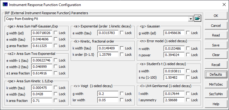
The IRF button in the three fitting options, and in the IRF Deconvolution option, controls the default starting estimates for the IRF parameters:

Please note that you may only need to use the first item in the dialog, the <ge> IRF, and possibly the second, the <e2> IRF, if you are modeling analytical peaks.

Most of the IRF parameters specify a first order kinetic (exponential) or probabilistic (half-Gaussian) instrumental distortion. The <k> IRF offers a variable kinetic order, and the <n> a probabilistic decay that varies from that of Gaussian. The <s> Student's t (also a Pearson VII peak shape and the <l> Generalized Normal (the right-side asymmetry of the LN4 peak) offer experimental models of instrumental tailing. The <ge>, <e2> and <pe> IRF include a third parameter which specifies the two components by an area fraction of the first component.

The initial values are defaults the program will use when automatically placing peaks to begin a fit, or to employ a Fourier deconvolution in a preprocessing step. The initial values in the program come from fits of high-resolution IC data which represent only a starting point. These values may or may not be especially applicable to your instrument. Although these are only starting estimates for an iterative fitting process, you should set these values as close to the expected fitted values as possible. The fits will be faster, and this also minimizes the possibility of fits where the global minimum (the optimum solution) is not automatically achieved.

Assigning IRF Default Parameter Values

Use the dropdown to select any fit from the current file. The IRF from that that specific fit will be shown with the average values of the IRF parameters across all data sets fitted. The count of values in the average will also be shown. Simply select the fit to insert this value into into the fields associated with that specific IRF.

Use the Select a Different Data File button to use fits stored in a different PeakLab file as a source of the IRF values.

Options

The Save option can be used to save configuration [irf] file to disk containing these IRF starting estimates. This option allows this specific IRF configuration to be recalled at any time. A PeakLab [pfd] data file automatically saves a current IRF configuration and that is used when a given pfd file is opened. Those values will be overridden when the Read option is used to open one of these [irf] configuration files. When such an IRF configuration is imported, all values in the dialog are updated.

The Clear option erases the values in all of the fields.

The Recall option restores the values from the current [pfd] file.

The Defaults option restores the initial program defaults based on this high S/N IC data.

The MinToSec option converts the time-based IRF parameters from a minutes to a seconds time scale. The SecToMin option does the reverse, converting all x-scale parameters from a seconds time scale to a minutes one. In general, you will probably find it easiest if you use only a minutes or seconds time scale. The program's Transform Data option can easily convert the time scale once the data have been imported.

The Instrument Response Functions

Convolution models were created for the following kinetic and Gaussian response functions (a₄, a₅, and a₆ are used as the IRF parameters):

	First Order Exponential <e>
	Sum of Two First Order Exponentials <e2>
	Convolution of Two First Order Exponentials <e2x>
	Half-Gaussian <g>
	Sum of Two Half-Gaussians <g2>
	Convolution of Two Half Gaussians <g2x>
	Sum of Half-Gaussian and First Order Exponential <ge>
	Convolution of Half-Gaussian and First Order Exponential <gex>
	Sum of Kinetic Order 1.5 and First Order Exponential <pe>

Convolution models were also created for the following response functions with adjustable shapes (a₄ and a₅ are used as the IRF parameters):

	Variable Order Kinetic <k> a₅=order, Exponential: a₅=1, bounded a₅ <1
	Symmetric Gen. Gaussian <n> a₅=power, Exponential: a₅=1, Gaussian: a₅=2
	Student’s t <s> a₅=DOF, Lorentzian a₅=1, Gaussian a₅->Infinity
	Asymmetric Gen. Gaussian (LN4 parameterization) <l> a₄= FWHM a₅= 1-Half-Height Asymmetry, Gaussian a₅ ~ 0 a₅¹0)

For spectral models, especially for asymmetric XPS peaks, there is also a Voigt IRF. Typically, one fits a Voigt<v> where the IRF is a right-sided Voigt with different Gaussian and Lorentzian widths to account the asymmetry. Here as well a₄ and a₅ are used as the IRF parameters:

IRF DIALOG11.PNG

Asymmetric Voigt (Gauss and Lorentz widths parameterization)
<v>
a₄=Gaussian width, a₅=Lorenzian width

The Most Effective Chromatographic Instrument Response Functions

We report IRF Model Fit results from a study where we compared the three IRFs we found most effective for fitting the IRF in analytic non-gradient LC peaks.