PeakLab v1 Documentation Contents            AIST Software Home            AIST Software Support

Modify GLM Data Matrix

The Modify GLM Data Matrix items process an imported data matrix and create a revised data matrix in a single step. The following options are available:

Generate Unit X-Spacing Data Matrix...

This option will use a constrained cubic spline interpolant to generate spectra with a unit x-spacing.

This is useful if you want the spectra in integer wavelengths. The column header for the X-variables will need to consist of numeric wavelength or frequency values.

Generate Center of Mass GLM Data Matrix...

This option will compute a center of mass predictor matrix.

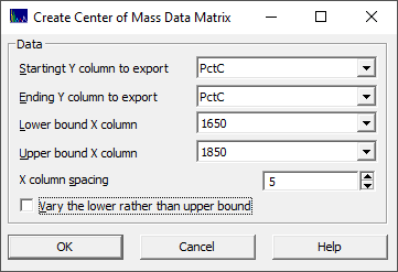
Because this option does not alter the Y or dependent variables, you must specify which of the Y variables you wish to place in the new data matrix. You must also specify the lower and upper bound for the center of mass computations. You must also specify the X-column spacing to be used. There is also an option to vary the lower bound rather than the upper bound.

In this example, we assume the pertinent spectral information begins at approx. 1650 nm and ceases at about 1850 nm. The computations then proceed as follows. The first column in the new data matrix will be 1652.5, the average of the 1650 and 1655nm wavelengths. A center of mass is computed for the information between 1650 and 1655. If this is 1652.4, the value in this first predictor will be -.1 and the process is then repeated for 1650 and 1660 (increasing the upper value by the 5nm column spacing specified). Here the midpoint is 1655. If the computed center of mass is 1655.1 for the 1650-1660 information, the value in this second predictor will be +.1 and this continues until the range between 1650 and 1850 is processed. If the center of mass for this last predictor is 1755, then a value of +5 is inserted into the 1750 predictor.

In this export, one new predictor matrix is written to the folder location of the imported file containing the original data matrix. It will have an appended string in the file name similar to _CtrMass1650-1850-0. The 0 specifies the upper bound is varied. If 1, the lower bound is varied and the upper, in this case 1850, is held constant.

This is an elaborate procedure that uses a constrained cubic spline to interpolate the raw data and root finding algorithms. You should not use this approach for any estimation where you need a simple model fully independent of PeakLab's analytics.

The generated center of mass data matrix will look similar to the above, typically small values around zero.

Generate Cumulative GLM Data Matrix...

This option will compute a cumulative predictor matrix.

This is analogous in most ways to the center of mass procedure, except that cumulatives between 0.01 and 0.99 of the specified range are computed for an X wavelength or wavenumber band that is held constant.

In this example, we again assume that all pertinent spectral information rests between 1650 nm and 1850 nm. The computations then proceed as follows. The first column in the new data matrix will be 1650+0.01*200=1652. A 0.01 cumulative of the 1650-1850 area is computed and the difference between this value and 1652 is placed in this first predictor. The process is then repeated for 1650+0.02*200=1654. The 0.02 cumulative's difference with 1654 is placed in this second predictor. The last predictor is 1650+0.99*200=1848 and the difference between the 0.99 cumulative's value and 1848 is placed in this last predictor.

As with the center of mass option, one new predictor matrix is written to the folder location of the imported file containing the original data matrix. It will have an appended string in the file name similar to _Cumulative1650-1850.

This is similarly an elaborate procedure that uses this same constrained cubic spline to interpolate the raw data and root finding algorithms for the cumulative. Again, you should not use this approach for any estimation where you need a simple model fully independent of PeakLab's analytics.

Generate Random Sampling GLM Data Matrices...

Although the full permutation GLM modeling includes random sampling predictive errors, these will be estimated for models which did well with the full set of data used in the modeling. The built-in random sampling predictive errors will effectively estimate the effect of lost bracketing of the modeling problem with the repeated random omission of a specified count of test data sets, but the model which will be evaluated will be one that performed especially well with all of the data. You can use this option as a rigorous test of the full permutation direct spectral fitting process.

This option will generate two randomly generated data matrices from the data set for each of the number of random sets specified. In the above example, a test set of 150 randomly selected samples is crated, and the remaining 151 samples are placed in the the modeling set. These will be written to the folder location of the imported file containing the original data matrix. The model files will have a "_1Fit", "_2Fit", etc appended to the name and the test files will have a "_1Pred", "_2Pred", etc. appended. In this example ten model files are generated for fitting, and ten test files are generated for prediction. With billions or even trillions of possible permutations of X-predictors in the models, you should expect to see different models in the best fitted list.

There is a Specific Models option in the GLM fitting procedure that can be used to force a specific model to be included in the retained list. You will need to use this option if you want to evaluate how well a specific model performs for prediction relative to all other possible models.

Generate Principal Component GLM Data Matrices...

This option will generate separate a principal component data matrix which can be independently fitted.

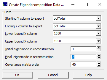
You must specify the Y-variable starting and ending column locations and the starting and ending column for the spectra. You must also specify the initial and final eigenmode for the reconstruction as well as the matrix order for the lagged covariance matrix.

Because there are edge effects in eigendecomposition, you should specify at least the matrix order of points on each side of the modeling band. For the default covariance matrix order of 40, you should specify at least 40 x columns prior and 40 x columns after the data that will be used for the modeling.

The algorithm used is the CovM FB (covariance matrix forward-backward) procedure, the covariance matrix equivalent of processing a forward-backward prediction data matrix.

The first step in an eigendecomposition is always the creation of a matrix that uses lagged copies of subsets of the data series. This can be a straightforward data or trajectory matrix, such as the forward prediction, backward prediction, or forward-backward prediction matrices used in autoregressive modeling, or one of several methods can be used to construct a covariance matrix from lagged copies of the data. The covariance data matrices are rectangular, and SVD is used to extract the eigenvectors and singular values.

Establishing the eigendecomposition order for harmonic signals in the absence of noise is a simple matter. Two eigenmodes are minimally needed to fully describe one oscillation. These oscillatory components can be harmonic, such as undamped or damped sinusoids, sawtooth, and others. Or they can be anharmonic, oscillations where the model is not readily apparent. As discussed in the Modeling FTNIR Spectra white paper, eigendecomposition will not separate overlapping peaks.

If eigendecomposition is being used to separate signal from noise, a higher order model is needed to account for the oscillations introduced by noise. To achieve a reasonable signal-noise separation within an eigendecomposition, it is necessary to use a high enough order so that the primary eigenvectors span only signal space. Further, when isolating components, the partitioning of component signals into different eigenmodes is usually enhanced by higher orders. We have found a matrix order of 40 to be close to optimal.

If you specify all of the eigenmodes in the reconstruction, this will produce an exact reconstruction of the input data.

The new data matrix will be written to the folder location of the imported file containing the original data matrix. For the above example, the file will have an "_Eigen(1_2_40)" appended to the file name as well as the _1550_1950 wavelength band.

Note that there is a To n principal components option in the GLM fitting procedure that addresses principal components directly in the matrix computations of the estimated parameters. That would allow, for example, eight predictor models to fit to a specified maximum of six principal components. The principal components are extracted in the fitting procedure as opposed to the raw input data.

Transform Current GLM Data Matrix...

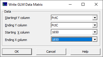
This option will modify the spectra in the data matrix per any user defined transform you wish to apply. To create a transformed data matrix, you must first specify the X and Y columns for the new data matrix:

The spectral data in the X columns are changed by the transform. All rows, all spectra, are processed.

The Y columns containing the dependent or reference variables in the data matrix are copied unchanged to the new matrix in this procedure. They cannot be modified using this procedure.

Once this is done, you will see the program's Transform Data dialog.

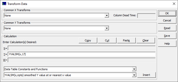
This is the Transform Data procedure in the main peak fit transform, except that here it is applied to the spectra in the GLM data matrix in order to produce a new matrix. Only the Y formula field will be available.

For the formulas in this procedure, the X values are fixed, the wavelengths or wavenumbers that appear in the header of the data matrix file. The Y values are the values of the spectra at each wavelength or wavenumber, this for each of the X columns of wavelengths or wavenumbers specified. These spectral values are the Y values modified by the transform.

In most instances, you will probably use the Data Table Constants and Functions as in the following examples:

Y=(Y-YMEAN)/YSTD - converts each spectrum in the data matrix to a mean=0, standard deviation=1 normalization
Y=MINLINBL(x,y,1640,1680,1830,1870) - for each spectrum, finds the minimum between 1640 and 1680 on one side of the data, between 1830 and 1870 on the other, constructs a linear baseline between these points, and then subtracts this baseline from the data, zeroing all negative values.
Y=YVALSM(x,17) - each spectrum is processed through the Savitzky-Golay quartic smoothing procedure using a 17-point window (PeakLab's default smoothing algorithm)
Y=YVALD2(x,23) - each spectrum is processed through the Savitzky-Golay quartic D2 (second derivative) smoothing procedure using a 23-point window (PeakLab's default D2 algorithm)

A new transformed data matrix is written to the folder location of the imported file containing the original data matrix. It will have _transform appended to the file name. You should replace this with a description of the transform useful to you.

A transform can be quite simple and that which can be as easily done in modifying the data matrix in Excel. It can also be more complex as in the above examples. As a caution, be careful when modifying the data matrix. Direct spectral fits rely on spectral magnitudes. Any transform that alters the signal, such a normalizing all spectra to unit area, may destroy a portion of the deterministic information in the data.

Create a GLM Data Matrix with Custom Predictors...

This option allows you to create a data matrix with a custom set of predictors.

Here also you must first specify which columns are X and which are Y:

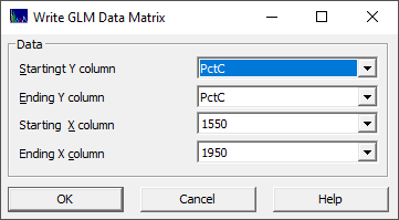
You will then see a dialog where you can enter your custom predictors:

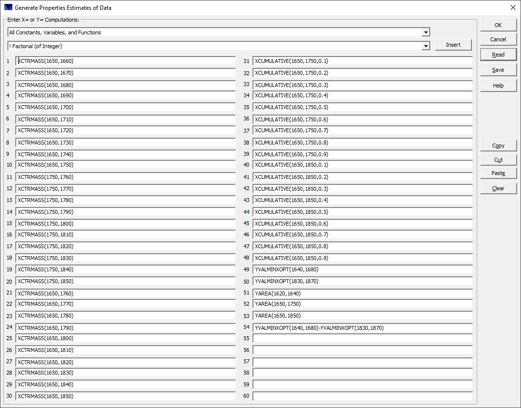
This example produces a mixed set of center of mass and cumulative predictors and a few items that might possibly be useful for normalization. All apply only to the predictors, the X-variables in the GLM modeling. Note that it is the spectral Y values that are being specified and computed (the spectral X values, the wavelengths or wave numbers, are not changed).

This is the same option available from right click menu item Export Data Property Computations in the main program window.

One new transformed data matrix is written to the folder location of the imported file containing the original data matrix. It will have _Predictors appended to the file name. You should replace this with a description of the predictor set. In all likelihood, you will need PeakLab to generate this matrix, depending on the complexity of the predictors.