Fit GLM Models

PeakLab v1 Documentation Contents AIST Software Home AIST Software Support

Fit GLM Models

Once the Import Data Matrix | Import Spectroscopic Data Matrix... item in the Model menu is used to load a spectroscopic modeling data matrix into the program, the Fit Full Permutation GLM Models... option is available for fitting full-permutation GLM models and for fitting smart stepwise forward models which use the full permutation models as their starting point.

This option is used to fit known analytic values, such as those acquired from chromatographic analysis, to spectra where the relationships are far from clear. The PeakLab full permutation GLM models are an alternative to the PLS (partial least squares) and PCR (principal component regression) procedures traditionally used to 'unscramble' the spectral information and generate viable predictors of the analytic quantities.

Please see the separate topic of Full-Permutation GLM Modeling for a complete description of the benefits and drawbacks of direct spectral modeling.

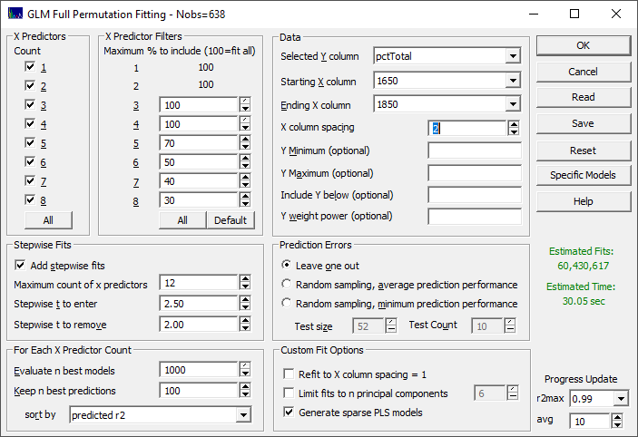
When you open this fitting procedure, you will see all of the options available to the algorithm in a single dialog.

X Predictors

The full-permutation fits can be specified for 1, 2, 3, 4, 5, 6, 7, and 8 total predictors. The default is to fit all counts of predictors. You can use the All button in this section to select all of the predictor counts in a single step.

X Predictor Filters

Full-permutation fitting can vary from requiring mere seconds to that which exceeds a human lifetime based on the number of x predictors used and the trimming of non-productive wavelengths or frequencies as the count of fitted predictors in increased. The defaults specify 100% of all permutations through four predictors, and then a successive trimming of non-productive predictors as the count of predictors increase. This will, in general, produce far faster fits. You can set these defaults in a single step using the Default button.

If the count of x-predictors is small enough, you may want to fit all permutations without filtering. You can remove the filters to fit all permutations, by clicking the All button in this section.

When the filters are changed upward to include a higher percentage of predictors, you will want to look very carefully at the Estimated Time and the Estimated Fits which will change with these filters. If you see these displayed in a red color, you will probably not wish to proceed at the current settings.

Stepwise Fits

In PeakLab's full permutation fitting, the stepwise fits are not the forward or backward models with which you may be familiar. These are fits which begin with the best of the full-permutation fits and where it is attempted to add one or more additional predictors to those fits using the traditional stepwise type of entry and removal criteria. Here you specify the maximum count of predictors which are permitted, and the |t| to enter and remove a parameter. In most instances, the defaults of a maximum of 12 predictors and a |t| to enter of 2.5, and a |t| to remove of 2.0 should be sufficient. When the |t| to enter is increased, it is harder for an additional predictor to be accepted and when the [t] to remove is increased, it is harder for a given predictor to remain in the model.

In general, you will likely see the best stepwise fits arising from the full permutation fits that are close to optimal. Typically, the stepwise procedure adds at most just a few further predictors relative to the full permutation fit.

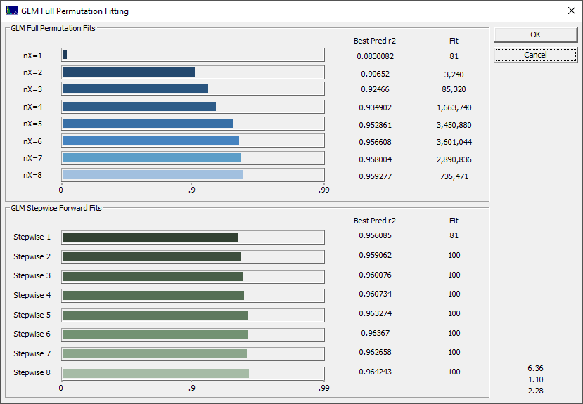
One purpose of the stepwise fits is to extend the models beyond the full permutation limit of eight predictors. Fits with nine or more predictors will exclusively be stepwise algorithm fits.

The stepwise algorithm is significantly changed from those used in statistical software packages. The enhanced PeakLab stepwise fitting algorithm will do an extensive search multiple times through all of the predictors in an effort to find the optimal additional ones. Tens or even hundreds of thousands of exploratory fits may internally occur in generating a single stepwise fit.

Please note that the X Predictor Filters do not apply to the new predictors added in the stepwise fitting procedure. All predictors are evaluated for the additional parameters in the stepwise algorithm. Even if the filter locks out certain GLM permutations, the stepwise procedure may still find those models. This is why you may see a stepwise 8-predictor fit, for example, that does not appear anywhere in the best 8-predictor full permutation GLM fits. Such a fit may have been built on a 7-predictor core model where this 8th predictor happened to be one that would have been excluded in the 8-predictor filtered subset.

When a stepwise fit replicates a full permutation GLM (general linear model) fit, both fits will appear within the model list. One will have a "GLM" prefix, the other a "Step" prefix. These should be equivalent to the full decimal places displayed in the goodness of fit estimates.

Retained Models

As a practical matter, you do not want to save or inspect a billion different fits. For each of the predictor counts, only the n best will be evaluated (Evaluate n best models). The maximum is 1000, the default.

The best models are based on the model (estimation, calibration) r² goodness of fits, but these are then further evaluated for prediction performance where you can specify the count of the best predictive models to be retained. The default to be kept (Keep n best predictions) of each count of predictors is 100. You can retain up the full count that were evaluated, invalidating any specified prediction sort, but we recommend limiting the model list to just the best performing models with respect to the prediction. The defaults also keep the total count of models in the vicinity of 1000.

You can also specify the prediction metric that will be used for this retention of models (sort by). The default is the predicted r². Other options include the standard error, the F-statistic, and three different well-respected information criteria. The retained models can also be based on a sort by overall average or median prediction error, or by the average prediction error in any one of the five quintiles of the Y-data.

Data Specification

Here you must specify the Selected Y column for the dependent variable being modeled as well as the Starting X column and Ending X column.

The X-column spacing is probably the most crucial item in the dialog. In general, you do not want to fit a high sampling rate of spectral information. If you see two adjacent wavelength or wavenumber columns with offsetting high-positive and high-negative parameters, you are fitting noise. This is often seen in traditional stepwise regression algorithms. If you use PeakLab to fit the spectral data to Gaussians, and you see Gaussian widths of 20 nm, for example, a 10 nm model x-spacing is likely all you will need. Those 10 nm spaced wavelengths can be subsequently refined to a 1 nm density with virtually no computational cost using the Refit to X column spacing=1 option described below.

In the example reflected in the above graphic, there are 201 spectral NIR wavelengths in the starting and ending columns specified and the default filtering has been selected. A 2 nm x-spacing (every other column) is shown with an overall fit time of 30 seconds and 60 million models to be fitted. If this 2 nm is changed to 1 nm, the time will change to 1.07 hours and 7.6 billion models to be fitted. If the filters are then removed at this 1 nm spacing, the estimated time becomes 1.1 years and 60 trillion models fitted.

Please refer to the white papers Modeling UV-VIS Data, Modeling FTNIR Spectra, and Modeling NIR Field Site Data for real-world examples where this column spacing is determined by peak fitting the spectroscopic data and by matched convolutions using very high resolution reference spectral data.

The Y Minimum is optional. If specified, all Y-data observations below this value will be omitted from the fitting.

Similarly, the Y Maximum is optional. If specified, all spectra with a higher Y-value will be omitted.

The Include Y below is useful if you specify a narrower Y range, but you want to help the linear model better know where the zero rests. If you specify a value for the Y-below, all observations below this Y value will be included irrespective of the Y-band specified. Typically, these samples will be your zero or near-zero references.

Weighting is useful to seek to give a uniform influence across a wide dynamic range of Y-values. The Y weight power is is optional. The default is unweighted least-squares. If a power is specified, weights will be automatically generated and applied to the fitting. A weight of one will apply an inverse weighting. A weighting of 1.1-1.3 is typically about right for least-squares problems where the Y-values span a couple of orders magnitude. This weighting will increase the errors in the highest Y-valued observations, and since these are often the values most accurately predicted, you can realistically expect to see a diminished r² of prediction with weighting.

Prediction Errors

The default estimate of prediction error is Leave One Out. In this example, there are 638 separate spectra (data observations). Leave One Out will perform 638 separate fits, each leaving out one of the 638 samples. There is then an error computed for the one observation that was omitted. The 638 different prediction errors are used to generate a predicted goodness of fit. This methodology does not significantly impact the bracketing of the model data, but it will reflect degraded predictions arising from overfitting.

There are two options for Random sampling prediction errors. These are identical procedures except one reports the average prediction performance, and the other reports the minimum prediction performance as a kind of worst-case scenario. You must specify a test size and a test count. The default test size is 1/3 the total sample size and the default test count is 10. In a random sampling prediction estimate, the bracketing of the fitting problem will be diminished and the predictions will correspondingly suffer, especially on observations in the test set that had represented this bracketing. The random sampling prediction errors will almost universally be higher than the Leave One Out errors.

Unit Spacing Resolution

The Refit to X column spacing=1 option adds a final fitting optimization that fits all of the adjacent columns next to a predictor which were excluded from the fitting by the specified X-spacing. If a 5 nm spacing is specified for the fitting, and a 1700 nm predictor is used in the model, this means that additional fits will be made with 1698, 1699, 1701, and 1702 nm for this predictor. If an overall improvement in goodness of fit is realized, the 1700 nm predictor will be replaced with the one offering the better performance.

Principal Components

The To n principal components recognizes that at a certain point, the eigenmodes will consist mostly of noise whose fitting will only distort or harm the predictions. This principal component processing occurs in the actual matrix computations of the fitted model, not in preprocessing the original data. Using this option, you can limit the principal components to signal-bearing information. If, for example, this value is set to 6, then all models with 7 or more predictors will use just the first 6 principal components of the eigenmatrix in estimating the coefficient values of this higher count of predictors.

Note that this is not PCR (principal component regression). PCR is analogous to PLS (partial least squares) regression, except that the indirect or latent factors are based on principal components rather than correlations between the Y-values and the spectra. This option in PeakLab's fitting is still a direct spectral fitting method. It simply uses a matrix procedure where the higher eigenmodes represent principal components which can be treated as noise, and as such are not allowed to influence the estimation of the fitted coefficients. In PeakLab's principal component fitting, the eigendecomposition is used only to separate signal and noise, and thus avoid overfitting by an in-situ removal of the noise from the fitting.

Note that the S/N separation occurs only in the computation of the predictor parameters. Since the data are unchanged, the goodness of fit will not reflect any form of noise reduction.

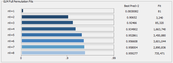
You can use the progress update to see where the predictions start to level off with respect to increasing predictor count. In the above example, there are dramatic improvements through six predictors, and there is shown little to be gained beyond six predictors. In this example, if you are doing principal component fits, five or six principal components are reasonable.

Sparse PLS Models

The Generate Sparse PLS Models will add 'PLS-like' models where the most significant direct spectral models are integrated into a weighted average prediction that uses a higher count of predictors.

The PLS (Partial Least Squares) algorithm works by an iterative set of factor (synthetic variable) extractions that use linear correlations between the dependent variable and every wavelength (WL) specified in the modeling. One of the distinguishing properties of this indirection, fitting derived factors instead of the spectra directly, is to effectively include in the model every WL in the prediction band to some degree and estimating a coefficient for its contribution to the overall predicted value. While direct spectral modeling precludes the generation of a coefficient for every WL in the predictors, sparse PLS models will offer a higher number of component WLs.

You can think of sparse-PLS models as 'PLS-like' insofar as they will offer a collection of WLs in the modeling band. Those will be sparse, however, in contrast with the PLS algorithm which includes every predictor in the modeling.

A sparse PLS[nsig,navg,npred] model is one where the most nsig significant predictors produce an optimal WL set, and it is populated with navg models, each consisting of npred predictors. You can readily equate the npred predictor count with a factor count.

In a PLS model, you will see something akin to PLS[15,35,8]. This means that the model consists of 15 predictors (15 wavelengths, 16 estimated coefficients). These will be the 15 most significant predictors in the retained 8-predictor models. This overall model will have been built by the statistical goodness of fit weighting of the 35 direct spectral fits of 8-predictor models which are a subset of these 15 significant wavelengths.

As to whether or not the additional predictors offer a more stable prediction, it is certainly possible. We can only point out the obvious tradeoff of more WLs to soften an anomaly at any given predictor, but a greater count of predictors where such anomalies might appear. The assessment might wisely be based on whether or not trace contaminants, as well as trace amounts of other species that may have been weakly represented or absent in the model data, might be likely to occur. In our experience, sparse-PLS models offer slightly better prediction performance relative to the optimum PLS or PCR models, and they will do so with far fewer predictors, and with each assured significant in a direct spectral modeling.

Because this option only assembles existing models, it adds virtually no additional time to the modeling process.

Specific Models

It is possible you may wish to ensure a given model is always fitted and included in the retained models. You can use the Specific Models button to import a txt ASCII file containing the models you want to force within the fitting.

Here is an example file:

5,1650,1675,1745,1785,1830

5,1660,1675,1735,1785,1830

5,1660,1675,1735,1785,1840

There is one line for each model. The first value is the predictor count, and the additional values are the column labels for the predictors, typically the wavelengths or wavenumbers. When importing such a Specific Models file, the forced models will be highlighted in the model list.

You can manually create the file or use the Add Current Model to Always Included Model File... option in the Model List window's File menu.

Note that this option will only process the models at the wavelengths in the original X-spacing. If you use the Refit to X column spacing =1 option to further refine the fit predictors, those refined wavelengths will not be applicable to this option since they do not occur in the actual full permutation fitting.

Saving and Recalling Configuration

Use the Save option to save the current fit configuration to disk, and the Read option to import a previously saved configuration. The Reset option will restore all defaults.

Progress Update

These settings control the progress dialog that is displayed during fitting. You can set the maximum r² (r2max) to be shown in the progress bar as well as the number of best fits averaged (avg) in the values shown.

Saving the Fit to Disk

When the fitting is finished, click OK and enter a name for the GLM Fit information to be saved to disk. This saves all fits retained to a binary file with a .bin extension.

A .bin GLM fit file can be loaded in a single step n the Model menu's Import Model Fits, including the automatic import of the data used for that particular fitting. This save of all fit information to disk is required in order for the fit to be available at any future time. If you Cancel this save of the fit, you will still see the GLM Review for the fit, but you will need to repeat the fit if you wish to subsequently revisit the fitting.