PeakLab v2 Documentation Contents R2N Software Home R2N Software Support
The Quest for a Universal Chromatographic Fit
Over the course of the five years PeakLab was in development, much came to light that helped us to better grasp the concept of an ideal chromatographic nonlinear fit. In simplest terms, an ideal chromatographic non-linear fit was seen to require:
(1) A model that was capable of accounting nearly all of the variance in the data while retaining statistical significance in all fitted parameters, and where each of the components of that model was in line with prevailing theory. The model would need to manage all types of chromatography, LC and GC, including gradient HPLC and preparative shapes.
(2) A fitting procedure that would manage such a complex model swiftly and efficiently, and which resolved the global solution in the iterative optimization in a single step requiring no user intervention.
(3) A certainty we 'got it right', that everything that could be estimated by a statistical modeling procedure was being fitted. As a test, we wanted to be able to fit higher concentrations with much more strongly fronted and tailed shapes and see equally effective fits. We also wanted to see gradient HPLC peaks and higher overload preparative shapes fitted by the same models, ideally to the same measure of efficacy.
What Would an Ideal Fit Look Like with Respect to Goodness of Fit?
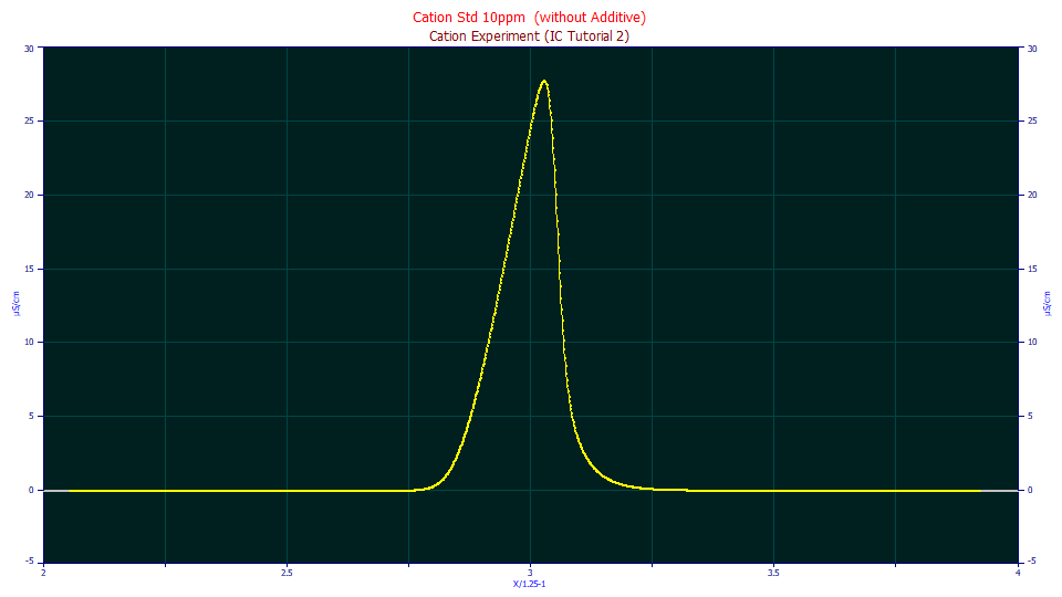
We will use one of the samples from the Chromatographic Experiments tutorial, one that has an good S/N and no impact from an additive:

We can generate a Fourier spectrum of the data that isolates the power where the noise in the data begins and how many significant figures exist where all determinacy is lost:
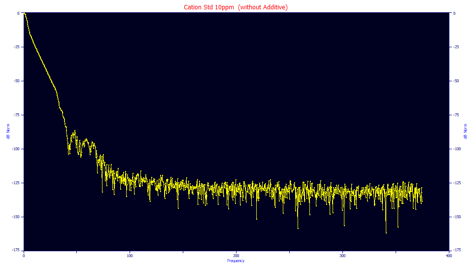
The noise floor begins at about -120 dB and finishes at the highest frequencies at about -130 dB. This corresponds to approximately six significant figures of information. The sixth significant figure in the data is likely to be the equivalent of random noise.
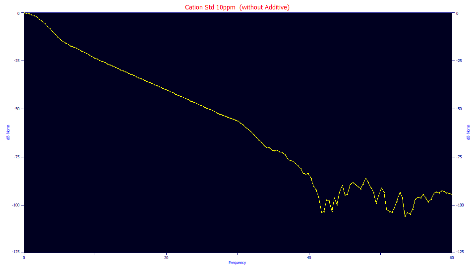
If we zoom-in, we see the noise starting at about -80 dB both in the decay and in the first oscillation. This corresponds to approximately four significant figures of information. This means the fourth significant figure should be attainable to full accuracy. For the count of points in this data set, this would be an F-statistic of 10^8 or 100 million. Using this loosely as a benchmark, we can say a 'perfect' fit would have every parameter significant, and a goodness of fit F-statistic of at least 100 million. Since the noise only begins at the -80 dB threshold, we could easily enough assert a higher F-statistic, perhaps closer to 10^9, one-billion, as being the target for a 'perfect' fit to this real world data.
The GenHVL<ge> Fit
If we fit the data to an HVL once-generalized chromatographic peak model with the <ge> IRF, the sum of half-Gaussian and exponential distortions, we see the following:
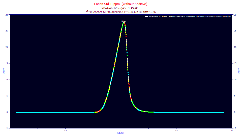
Fitted�Parameters
r2�Coef�Det�� DF�Adj�r2���� Fit�Std�Err�� F-value������ ppm�uVar
0.99999854��� 0.99999853��� 0.00698952��� 1.3617e+08��� 1.46243271
�Peak�� Type�������� ������a0���� ������a1���� ������a2���� ������a3���� ������a4���� ������a5���� ������a6���� ������a7����
����1�� GenHVL<ge>�� 3.81823449�� 2.87894324�� 0.03850284�� -0.0058968�� 0.01509544�� 0.00507165�� 0.04195172�� 0.65914916��
Parameter�Statistics
Peak�1�GenHVL<ge>
�Parameter����� Value������� Std�Error��� t-value����� 99%�Conf�Lo�� 99%�Conf�Hi�� P>|t|
���������Area�� 3.81823449�� 0.00017319�� 22046.9454�� 3.81778778��� 3.81868121��� 0.00000
�������Center�� 2.87894324�� 0.00016563�� 17382.1215�� 2.87851602��� 2.87937045��� 0.00000
��������Width�� 0.03850284�� 2.7689e-05�� 1390.56223�� 0.03843142��� 0.03857426��� 0.00000
�����Distortn�� -0.0058968�� 2.4275e-06�� -2429.1650�� -0.0059031��� -0.0058906��� 0.00000
�������Z-Asym�� 0.01509544�� 5.5308e-05�� 272.932932�� 0.01495278��� 0.01523810��� 0.00000
���������g-sd�� 0.00507165�� 0.00015753�� 32.1939309�� 0.00466531��� 0.00547798��� 0.00000
��������e-tau�� 0.04195172�� 3.4493e-05�� 1216.23128�� 0.04186275��� 0.04204069��� 0.00000
�������g-frac�� 0.65914916�� 0.00103868�� 634.604392�� 0.65647003��� 0.66182828��� 0.00000
For a 99% statistical significance (99% confidence the parameter is non-zero), with this count of data, the magnitude of the t-value, the ratio of the parameter estimate to its standard error, should be 2.5 or higher. Only the half-Gaussian narrow width component, which we know must approximate multiple effects, has anything other than an exceptional significance. Even the weakest parameter is well removed from this threshold of statistical insignificance. For the moment, we will postpone discussion of the assumptions associated with the least-squares confidence statistics.
The GenHVL<pe> Fit
If we fit the GenHVL<pe> model where the IRF's narrow component approximately models interphase mass-transfer resistances with an order 1.5 kinetic decay instead of the half-Gaussian intended to model axial dispersion, we see a slight improvement, an F-statistic of 145 million and 1.38 ppm error, but this a5 (k-tau) time constant parameter has slightly less significance. A <pe> IRF is harder to fit than the <ge> IRF since the long tail of the 1.5 power narrow width component will be more correlated with the higher width exponential. Note also that a7 (k-frac), the area fraction of this narrow IRF component, has a wider confidence band.
Fitted�Parameters
r2�Coef�Det�� DF�Adj�r2���� Fit�Std�Err�� F-value������ ppm�uVar
0.99999862��� 0.99999862��� 0.00678137��� 1.4466e+08��� 1.37662531
�Peak�� Type�������� ������a0���� ������a1���� ������a2���� ������a3���� ������a4���� ������a5���� ������a6���� ������a7����
����1�� GenHVL<pe>�� 3.82107931�� 2.88269228�� 0.03873919�� -0.0058753�� 0.01521039�� 0.00022985�� 0.04187664�� 0.55635860��
Parameter�Statistics
Peak�1�GenHVL<pe>
�Parameter����� Value������� Std�Error��� t-value����� 99%�Conf�Lo�� 99%�Conf�Hi�� P>|t|
���������Area�� 3.82107931�� 0.00022505�� 16978.9483�� 3.82049883��� 3.82165979��� 0.00000
�������Center�� 2.88269228�� 5.3479e-05�� 53903.2631�� 2.88255433��� 2.88283022��� 0.00000
��������Width�� 0.03873919�� 1.5543e-05�� 2492.35269�� 0.03869910��� 0.03877928��� 0.00000
�����Distortn�� -0.0058753�� 1.8227e-06�� -3223.4798�� -0.0058800��� -0.0058706��� 0.00000
�������Z-Asym�� 0.01521039�� 5.4004e-05�� 281.655247�� 0.01507109��� 0.01534968��� 0.00000
��������k-tau�� 0.00022985�� 7.9302e-06�� 28.9842808�� 0.00020940��� 0.00025031��� 0.00000
��������e-tau�� 0.04187664�� 3.3724e-05�� 1241.75128�� 0.04178966��� 0.04196363��� 0.00000
�������k-frac�� 0.55635860�� 0.00602294�� 92.3731858�� 0.54082325��� 0.57189395��� 0.00000
Limitations of Nonlinear Modeling
Just as we discussed in the topic Understanding PeakLab's models with respect to spectroscopy, there will be factors which can be modeled and those which cannot. Just as the two different kinds of Lorentzian broadening can't be identified in Voigt model fits, so does a similar argument apply to this narrow width IRF component in chromatography.
We know there are multiple narrow-width IRF effects, but non-linear modeling can only statistically manage a single representation of this IRF component. We successfully model nearly all of the variance that can be modeled, given the S/N of the system, using a single narrow width component. There is too little variance remaining to add a second narrow width component to the IRF and quantify both.
We cannot model the amount and width of a postulated half-Gaussian axial dispersion, the amount and width of a postulated interphase mass-transfer resistances through porous media, and the amount and time constant of a higher width first order system delay. In nonlinear peak fitting, we can only model the amount and width of one assumed form of narrow-width component, as well as the amount and time constant of a higher-width exponential.
Benefits of Nonlinear Modeling
For a spectroscopic peak, both natural and collision broadening have the same theoretical shape, the Lorentzian. The instrumental distortion typically has the same theoretical shape as Doppler broadening, the Gaussian. The convolution actually has a closed-form solution (in the complex domain), a lovely simplification, but fitting that convolution, the Voigt model, cannot distinguish the two types of Lorentzian spectral broadening, nor can peak fitting separate the IRF and Doppler sources of Gaussian broadening.
For chromatographic peaks, apart from this issue of insufficient information to process more than one narrow-width IRF, there is far less ambiguity. Each of the parameters in a PeakLab once-generalized model describes a unique feature of a peak:
a0 - the area (zero moment); fitting is the only way to quantify accurate peak areas when peaks are overlapped or there are small hidden peaks in the rise or decay of larger peaks
a1 - this will be the center of mass (first moment) of one of the deconvolutions with the impact of the IRF removed. This will be the 'true' peak center, and depending on the model selected, this can reflect or remove any concentration dependency. In a conventional integration, you see only the mode of the peak, and with the IRF's distortion altering the observed retention.
a2 - depending on model selected, this will be either a diffusion width (square root of the second moment) or a kinetic time constant, a width independent of the IRF and multiple-site binding effects; for a kinetic model, this will be the solute desorption time constant.
a3 - the concentration-dependent chromatographic tailing and fronting, the shape unique to chromatographic peaks that can only be realized by peak fitting; for the kinetic models, this will estimate the equilibrium constant for adsorption.
a4 - the zero-distortion density (ZDD) third moment asymmetry which likely accounts multiple-site kinetics. It is this parameter that allows a generalized chromatographic model to fit the HVL theoretical model, the NLC theoretical model, and all shapes between as well as those of a greater asymmetry as is routinely seen in chromatographic peaks. This a4 parameter is generally treated as a constant across all peaks.
a5 - the SD width or time constant of the narrow width instrument response function (IRF) component; its limited impact on peak shape requires this be specified as a half-Gaussian, for modeling axial dispersion, an exponential, for fast first order kinetic distortions, or as a 1.5 fractional order kinetic, to approximate mass-transfer resistances with a second order step in an overall sequence. While this a5 parameter is sensitive to run conditions and prep, the impact is usually small enough that this factor can be treated as constant across all peaks.
a6 - the time constant of the wider IRF component; always a first-order exponential, and generally very close to constant, independent of run conditions and prep, specific to the instrument flow path and detection.
a7 - the area fraction of the narrow component of the IRF; also very close to independent of process variables. This a7 parameter is also easily treated as constant across all peaks in the data.
Do We Have It Right?
One could make a strong argument with respect to the orthogonality of the parameters in the once-generalized chromatographic models. Parameters a0, a1, a2, and a4 correspond directly with the zero, first, second, and third moments of the zero distortion density (ZDD) upon which a generalized model is built. The a3 parameter is the concentration operator that produces the chromatographic tailing and fronting using this ZDD as its starting point. We cannot imagine a more compact optimum with respect to this orthogonality of moment-mapped parameters. In the twice generalized models, we do use one more parameter in the core model, but this corresponds directly with an adjustment to the fourth moment of the ZDD.
In a peak fit, there are ways to have a reasonable certainty of a correct model and an optimum fit. Because it is a statistical regression procedure with confidence statistics and probabilities, there are statistical metrics that readily catch incorrect models and overfitting. In the fits above, the probabilities (the probability of the values actually being indistinguishable from zero) are all 0. Again we will defer discussing the assumptions which underlie these confidence statistics. We will instead give several examples of what happens when fitting an incorrect or overspecified IRF or an incorrect core model.
Examples Where Parameter Significance Fails
Convolving Rather then Summing the Two Components of the IRF - An Incorrect IRF
We will start by fitting the same generalized core model, but the IRF will consist of the half-Gaussian and exponential convolving one another instead of summing together in a simultaneous distortion:
Fitted�Parameters
r2�Coef�Det�� DF�Adj�r2���� Fit�Std�Err�� F-value������ ppm�uVar
0.99643976��� 0.99642188��� 0.34474151��� 65,072������� 3560.24004
�Peak�� Type��������� ������a0���� ������a1���� ������a2���� ������a3���� ������a4���� ������a5���� ������a6����
����1�� GenHVL<gex>�� 3.69149765�� 2.89959539�� 0.04570381�� -0.0051920�� 0.01352180�� 0.00013341�� 0.00736533��
Parameter�Statistics
Peak�1�GenHVL<gex>
�Parameter����� Value������� Std�Error��� t-value����� 99%�Conf�Lo�� 99%�Conf�Hi�� P>|t|
���������Area�� 3.69149765�� 0.00829569�� 444.989798�� 3.67010010��� 3.71289521��� 0.00000
�������Center�� 2.89959539�� 0.00331705�� 874.149369�� 2.89103953��� 2.90815124��� 0.00000
��������Width�� 0.04570381�� 0.00100273�� 45.5794441�� 0.04311741��� 0.04829020��� 0.00000
�����Distortn�� -0.0051920�� 7.5952e-05�� -68.358426�� -0.0053879��� -0.0049961��� 0.00000
�������Z-Asym�� 0.01352180�� 0.00397407�� 3.40250724�� 0.00327125��� 0.02377236��� 0.00069
���������g-sd�� 0.00013341�� 1157.31869�� 1.1527e-07�� -2985.1394��� 2985.13966��� 1.00000
��������e-tau�� 0.00736533�� 0.00187375�� 3.93080002�� 0.00253226��� 0.01219840��� 0.00009
This is an example of how critical it is to get the IRF correct. We are fitting the same GenHVL peak model with only the IRF changed. We even use the same two IRF components, but in a convolution instead of a sum. The fit is poor, at least by contrast, an error of 3560 ppm, and the half-Gaussian width is statistically indistinguishable from 0. The grayed values in the table indicate a failed significance for a given parameter. This can occur with a model that is incorrect, as in this case, as well as with a model which is overspecified, when two or more parameters are strongly correlated and it becomes a mathematical tossup in terms of which portions of the variance each of these parameters capture.
Fitting an IRF with Two Narrow-Width Components - An Overspecified IRF
We will now fit an example of an overspecified IRF. We have created a GenHVL<gpe> UDF where the IRF is a five-parameter sum of a half-Gaussian and order 1.5 kinetic for the narrow component, and the same first order exponential for the higher width component. This is an example of fitting a model that describes two narrow width IRF components, the axial dispersion as a half-Gaussian and the mass transfer resistances with a 1.5 power kinetic decay. There are two additional IRF parameters, the additional narrow width term, and a second area fraction:
Fitted�Parameters
r2�Coef�Det�� DF�Adj�r2���� Fit�Std�Err�� F-value������ ppm�uVar
0.99999870��� 0.99999869��� 0.00658858��� 1.1919e+08��� 1.29760045
�Peak�� Type�������������� ������a0���� ������a1���� ������a2���� ������a3���� ������a4���� ������a5���� ������a6���� ������a7�� ������a8�������a9����
����1�� GenHVL<gpe>-udf1�� 3.82081148�� 2.87969655�� 0.03855468�� -0.0058916�� 0.01515923�� 0.00418343�� 0.00093313�� 0.04178429 0.58254686 0.09016889��
Parameter�Statistics
Peak�1�GenHVL<gpe>-udf1
�Parameter����� Value������� Std�Error��� t-value����� 99%�Conf�Lo�� 99%�Conf�Hi�� P>|t|
�����������a0�� 3.82081148�� 0.00028478�� 13416.8184�� 3.82007694��� 3.82154603��� 0.00000
�����������a1�� 2.87969655�� 0.00047178�� 6103.92815�� 2.87847966��� 2.88091344��� 0.00000
�����������a2�� 0.03855468�� 2.8851e-05�� 1336.33152�� 0.03848026��� 0.03862910��� 0.00000
�����������a3�� -0.0058916�� 2.8715e-06�� -2051.7479�� -0.0058990��� -0.0058841��� 0.00000
�����������a4�� 0.01515923�� 5.3469e-05�� 283.513409�� 0.01502132��� 0.01529715��� 0.00000
�����������a5�� 0.00418343�� 0.00026756�� 15.6353479�� 0.00349329��� 0.00487357��� 0.00000
�����������a6�� 0.00093313�� 0.00122949�� 0.75895921�� -0.0022382��� 0.00410442��� 0.44801
�����������a7�� 0.04178429�� 8.1879e-05�� 510.316549�� 0.04157309��� 0.04199548��� 0.00000
�����������a8�� 0.58254686�� 0.10733620�� 5.42731038�� 0.30568753��� 0.85940618��� 0.00000
�����������a9�� 0.09016889�� 0.11126955�� 0.81036448�� -0.1968360��� 0.37717378��� 0.41787
The fit does have a better r2 goodness of fit than either the GenHVL<ge> model with the half-Gaussian narrow IRF component, and the GenHVL<pe> model with the 1.5 order kinetic decay. The F-statistic, however, suggests a weaker description of the data, and more importantly, the 1.5 order kinetic time constant, a6, and the 1.5 order area fraction, a9, test as insignificant. This is why PeakLab limits all built-in IRFs to three parameters and no more than two components. There is not enough information in the data for two narrow width components to be realistically fitted.
Fitting a Core Model with a Fourth Moment Adjustment instead of a Third Moment Adjustment - An Incorrect Core Model
Here we fit a model where the kurtosis or fourth moment of the ZDD is adjustable, but where the third moment or skewness is constrained to be zero. The ZDD is thus symmetric and only the thinness or fatness of the tails is adjusted:
Fitted�Parameters
r2�Coef�Det�� DF�Adj�r2���� Fit�Std�Err�� F-value������ ppm�uVar
0.99999753��� 0.99999751��� 0.00908698��� 80,564,528��� 2.47183679
�Peak�� Type����������� ������a0���� ������a1���� ������a2���� ������a3���� ������a4���� ������a5���� ������a6���� ������a7����
����1�� GenHVL[Q]<ge>�� 3.81959030�� 2.88406266�� 0.03922594�� -0.0058327�� 1.94088791�� 0.00044012�� 0.04209852�� 0.64684284��
Parameter�Statistics
Peak�1�GenHVL[Q]<ge>
�Parameter����� Value������� Std�Error��� t-value����� 99%�Conf�Lo�� 99%�Conf�Hi�� P>|t|
���������Area�� 3.81959030�� 0.00022522�� 16959.7284�� 3.81900939��� 3.82017121��� 0.00000
�������Center�� 2.88406266�� 0.00070015�� 4119.21186�� 2.88225673��� 2.88586860��� 0.00000
��������Width�� 0.03922594�� 3.926e-05��� 999.129240�� 0.03912467��� 0.03932720��� 0.00000
�����Distortn�� -0.0058327�� 3.946e-06��� -1478.1241�� -0.0058429��� -0.0058225��� 0.00000
������Q-power�� 1.94088791�� 0.00029393�� 6603.15370�� 1.94012975��� 1.94164607��� 0.00000
���������g-sd�� 0.00044012�� 0.00117210�� 0.37549847�� -0.0025831��� 0.00346339��� 0.70735
��������e-tau�� 0.04209852�� 4.4059e-05�� 955.493268�� 0.04198487��� 0.04221216��� 0.00000
�������g-frac�� 0.64684284�� 0.49246444�� 1.31348131�� -0.6234006��� 1.91708632��� 0.18924
In this instance we fit the same IRF, and only the higher moment in the ZDD is changed. This [Q] ZDD is capable of reproducing the HVL, but not the NLC since its ZDD is the asymmetric Giddings. Here we see that we have an exceptional 2.47 ppm error, but both the half-Gaussian width, and its area fraction failed the significance testing. In the conventional analysis, we want a t-value > 2.5 and a probability of zero < 0.01. This is an example of how critical it is to get the ZDD correct.
Examples Where Parameter Significance Succeeds
Fitting a Twice-Generalized Core Model with Both Third and Fourth Moment Adjustments - An Extension to An Appropriate Core Model
If the orthogonality of moments translates to a lack of intercorrelation between the parameters, we should also be able to fit a twice-generalized model to full significance:
Fitted�Parameters
r2�Coef�Det�� DF�Adj�r2���� Fit�Std�Err�� F-value������ ppm�uVar
0.99999864��� 0.99999863��� 0.00673985��� 1.2814e+08��� 1.35884292
�Peak�� Type��������� ������a0���� ������a1���� ������a2���� ������a3���� ������a4���� ������a5���� ������a6���� ������a7���� ������a8����
����1�� Gen2HVL<ge>�� 3.81849882�� 2.87996856�� 0.03868929�� -0.0058778�� 1.98538288�� 0.01146987�� 0.00417975�� 0.04196685�� 0.66548681��
Parameter�Statistics
Peak�1�Gen2HVL<ge>
�Parameter����� Value������� Std�Error��� t-value����� 99%�Conf�Lo�� 99%�Conf�Hi�� P>|t|
���������Area�� 3.81849882�� 0.00016906�� 22587.0020�� 3.81806276��� 3.81893488��� 0.00000
�������Center�� 2.87996856�� 0.00021214�� 13575.8441�� 2.87942138��� 2.88051574��� 0.00000
��������Width�� 0.03868929�� 3.1929e-05�� 1211.72535�� 0.03860693��� 0.03877165��� 0.00000
�����Distortn�� -0.0058778�� 2.9055e-06�� -2022.9989�� -0.0058853��� -0.0058703��� 0.00000
������Y-power�� 1.98538288�� 0.00137469�� 1444.24106�� 1.98183706��� 1.98892871��� 0.00000
�������Y-asym�� 0.01146987�� 0.00034598�� 33.1514053�� 0.01057745��� 0.01236229��� 0.00000
���������g-sd�� 0.00417975�� 0.00020540�� 20.3492876�� 0.00364994��� 0.00470955��� 0.00000
��������e-tau�� 0.04196685�� 3.3052e-05�� 1269.73547�� 0.04188160��� 0.04205210��� 0.00000
�������g-frac�� 0.66548681�� 0.00136143�� 488.815224�� 0.66197519��� 0.66899843��� 0.00000
While the statistics confirm the third moment Y-asym and the half-Gaussian IRF g-sd width are the most weakly determined of the parameters, all test to full 99% significance without difficulty. The fourth moment parameter, Y-power, fits to 1.985 just shy of the 2.0 power of a Gaussian decay. Note that the F-statistic of 128 million for the twice-generalized model is less than the 136 million of the once-generalized model. In this instance, there is no statistical basis for using a twice-generalized model which also adjusts the fourth moment. We only note the stability of a fit where parameters which strictly adjust the specific moments are used. This twice generalized model fit is one with every parameter significant. It is simply not a 'better' model for this data. The F-statistic is used to select the most appropriate model for the data.
Fitting a Different Once-Generalized Model that Performs a Different Third Moment Adjustment
In this case, we will fit an alternative model that adjusts the third moment or skewness of the ZDD. The GenHVL[G] model uses the Skew Normal or GMG as the ZDD instead of the default generalized normal ZDD.
Fitted�Parameters
r2�Coef�Det�� DF�Adj�r2���� Fit�Std�Err�� F-value������ ppm�uVar
0.99999884��� 0.99999883��� 0.00623526��� 1.7111e+08��� 1.16383188
�Peak�� Type����������� ������a0���� ������a1���� ������a2���� ������a3���� ������a4���� ������a5���� ������a6���� ������a7����
����1�� GenHVL[G]<ge>�� 3.81848259�� 2.86191875�� 0.03643718�� -0.0052848�� 0.02150691�� 0.00501900�� 0.04194502�� 0.65928185��
Parameter�Statistics
Peak�1�GenHVL[G]<ge>
�Parameter����� Value������� Std�Error��� t-value����� 99%�Conf�Lo�� 99%�Conf�Hi�� P>|t|
���������Area�� 3.81848259�� 0.00015440�� 24731.5265�� 3.81808435��� 3.81888084��� 0.00000
�������Center�� 2.86191875�� 0.00013431�� 21308.3103�� 2.86157231��� 2.86226518��� 0.00000
��������Width�� 0.03643718�� 2.4197e-05�� 1505.83501�� 0.03637476��� 0.03649959��� 0.00000
�����Distortn�� -0.0052848�� 3.2396e-06�� -1631.2892�� -0.0052931��� -0.0052764��� 0.00000
���������G-sd�� 0.02150691�� 2.5111e-05�� 856.473158�� 0.02144214��� 0.02157168��� 0.00000
���������g-sd�� 0.00501900�� 0.00013860�� 36.2122220�� 0.00466150��� 0.00537650��� 0.00000
��������e-tau�� 0.04194502�� 3.0735e-05�� 1364.73281�� 0.04186574��� 0.04202429��� 0.00000
�������g-frac�� 0.65928185�� 0.00090713�� 726.779448�� 0.65694205��� 0.66162166��� 0.00000
In this case, we have a slightly better F-statistic, and thus potentially a better model for describing this specific data, although as you shall see shortly, this is not the case when a small measure of overload is present. In this fit, all of the parameters are statistically significant. This does illustrate that there is more than one way to model the ZDD asymmetry arising from multiple-site adsorption and other effects which directly impact the actual chromatographic separation. Both the logarithmic scaling of the generalized normal, and the half-Gaussian convolution of the skew normal, can produce a statistically viable picture of the intrinsic ZDD skewness. We selected the GenHVL's and GenNLC's generalized normal for the default once-generalized chromatographic models since it can fit both the HVL and NLC to a much higher precision than the data can be sampled, and as you shall see, it is appreciably more robust with respect to modeling wide ranges of concentration.
Fitting a Different Once-Generalized Model with Two Third-Moment ZDD Adjustments - A Possible Overspecification
In this fit we use the GenHVL[V] as the core model. The 'V' ZDD uses two third moment-adjustments, this logarithmic factor as well as a half-Gaussian convolution in the ZDD. It can be overspecified since there are two separate adjustments of the third moment skewness in the ZDD.
Fitted�Parameters
r2�Coef�Det�� DF�Adj�r2���� Fit�Std�Err�� F-value������ ppm�uVar
0.99999885��� 0.99999885��� 0.00619136��� 1.5185e+08��� 1.14667712
�Peak�� Type����������� ������a0���� ������a1���� ������a2���� ������a3���� ������a4���� ������a5���� ������a6���� ������a7���� ������a8����
����1�� GenHVL[V]<ge>�� 3.81854086�� 2.86127001�� 0.03625329�� -0.0051807�� 0.02337363�� -0.0031897�� 0.00445524�� 0.04195416 0.66326512��
Parameter�Statistics
Peak�1�GenHVL[V]<ge>
�Parameter����� Value������� Std�Error��� t-value����� 99%�Conf�Lo�� 99%�Conf�Hi�� P>|t|
���������Area�� 3.81854086�� 0.00015426�� 24754.0990�� 3.81814297��� 3.81893875��� 0.00000
�������Center�� 2.86127001�� 0.00021502�� 13306.8336�� 2.86071539��� 2.86182463��� 0.00000
��������Width�� 0.03625329�� 6.2735e-05�� 577.880863�� 0.03609147��� 0.03641511��� 0.00000
�����Distortn�� -0.0051807�� 3.6767e-05�� -140.90579�� -0.0052755��� -0.0050859��� 0.00000
���������G-sd�� 0.02337363�� 0.00062766�� 37.2393064�� 0.02175467��� 0.02499260��� 0.00000
�������Z-Asym�� -0.0031897�� 0.00108503�� -2.9397491�� -0.0059884��� -0.0003910��� 0.00334
���������g-sd�� 0.00445524�� 0.00028504�� 15.6301759�� 0.00372002��� 0.00519047��� 0.00000
��������e-tau�� 0.04195416�� 3.0661e-05�� 1368.33747�� 0.04187508��� 0.04203325��� 0.00000
�������g-frac�� 0.66326512�� 0.00196434�� 337.652224�� 0.65819836��� 0.66833187��� 0.00000
Although in this example, the significance of all parameters met the 99% limits, it only barely did so in the logarithmic adjustment represented in the Z-Asym parameter. The ppm is the best of the models, but again, one is at a threshold of significance in one of the parameters, and the F-statistic suggests that the model, while not overspecified per se, may be more complex than necessary. One should always use the simplest model that accurately represents the data, even if that model does not have the best r� goodness of fit. For model selection, we rely almost exclusively on the F-statistic.
Fitting a One Component IRF - An Insufficient Description of the IRF
In this next fit, we omit the narrow width component in the IRF and fit only the higher width first order exponential:
Fitted�Parameters
r2�Coef�Det�� DF�Adj�r2���� Fit�Std�Err�� F-value������ ppm�uVar
0.99934974��� 0.99934694��� 0.14727979��� 429,084������ 650.263870
�Peak�� Type������� ������a0���� ������a1���� ������a2���� ������a3���� ������a4���� ������a5����
����1�� GenHVL<e>�� 3.77081642�� 2.85630628�� 0.03159503�� -0.0063686�� 0.01236693�� 0.02538398��
Parameter�Statistics
Peak�1�GenHVL<e>
�Parameter����� Value������� Std�Error��� t-value����� 99%�Conf�Lo�� 99%�Conf�Hi�� P>|t|
���������Area�� 3.77081642�� 0.00318714�� 1183.13488�� 3.76259566��� 3.77903719��� 0.00000
�������Center�� 2.85630628�� 0.00052933�� 5396.06983�� 2.85494095��� 2.85767161��� 0.00000
��������Width�� 0.03159503�� 0.00029123�� 108.489870�� 0.03084385��� 0.03234620��� 0.00000
�����Distortn�� -0.0063686�� 4.6122e-05�� -138.08015�� -0.0064876��� -0.0062496��� 0.00000
�������Z-Asym�� 0.01236693�� 0.00088629�� 13.9536428�� 0.01008088��� 0.01465298��� 0.00000
��������e-tau�� 0.02538398�� 0.00013983�� 181.531310�� 0.02502330��� 0.02574465��� 0.00000
Although all parameters are significant at the 99% threshold, note the much higher error, 650 ppm relative to values in the single digits. Each of the parameters is significant in the fitted model, but the model itself isn't a particularly good one. One wants a fit with close to zero error and full statistical significance in each parameter.
Confidence Statistics and Assumptions
In a typical regression analysis, one may capture 90% of the variance of the data. The remaining 10%, will consist of residuals (the difference between the data and fit at each point in the data). In such a fit, one wants the assumptions underlying the confidence statistics to be met. The normal statistical assumptions of 'IID' (independent and identically distributed) residuals, of a normal (Gaussian) density, are necessary to treat the statistics of the least-squares fit as valid. One does not want systematic trends in the residuals (the residuals should not be correlated across adjacent points), and the histogram of the residuals should consist of a normal density. If these requirements are not met, the confidence statistics are deemed inaccurate, and a more complex estimate of error, as realized by non-parameteric methods or a computationally intense bootstrap, is then used.
For a PeakLab fit where the unaccounted variance is 1 ppm, as in this example, the residuals will not consist of 10% of the variance or power within the data. In this instance, they represent just one part per million of the variance, .0001%, five orders of magnitude less than this 10%. It is our experience that PeakLab fits can be so close to complete, you can see as many different fits and error distributions as as you like simply by making exceptionally small differences in the intricacies of fitting the baseline in the baseline correction step. In fact, in the kind of baselines observed in higher concentration analyses, you can see differences as great as 100 ppm error vs 1 ppm simply by fitting a linear rather than non-parameteric baseline. A PeakLab fit to analytic chromatographic data will be such that the error you see will likely be a product of the accuracy of the baseline correction.
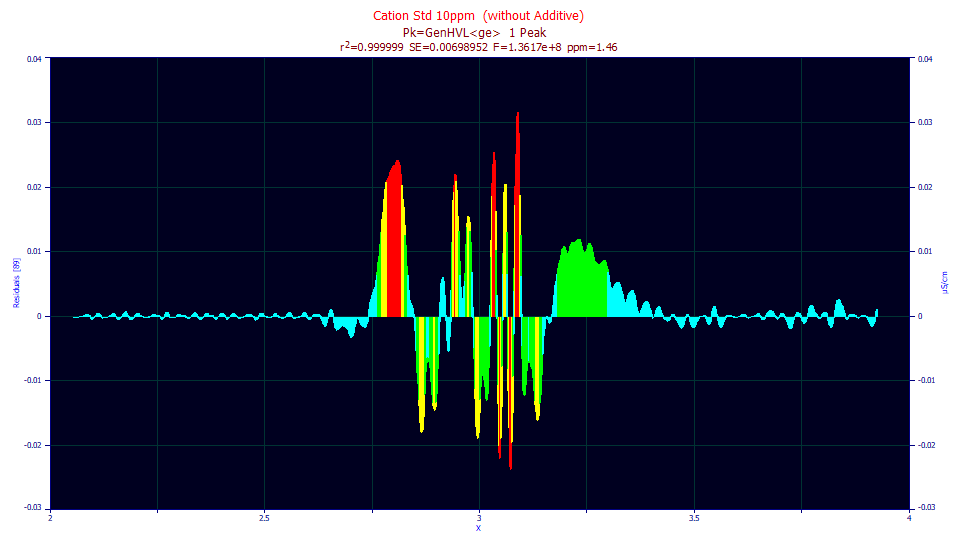
For the GenHVL<ge> fit the residuals show a strong systematic trend. One point's value is strongly correlated with the point prior and after. This is fully expected. We know we are not capturing the narrow width components of the IRF as they actually exist. We have made a simplification where a single component must be fitted for all narrow width IRF processes. Since we fit a single peak standard in this example, this systematic trend is not a baseline correction issue. The different systematic oscillations do correspond with that which is not being accounted in the model. If our model was 'perfect' at this 1 ppm error, we would see uncorrelated random residuals.
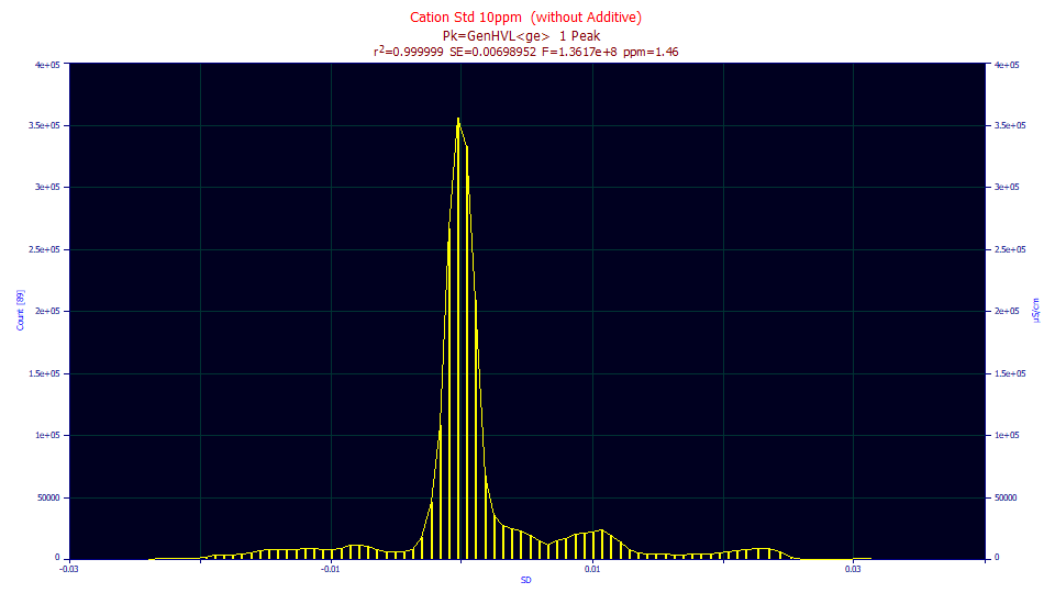
When systematic trends exist, the density of the residuals will seldom be Gaussian. For this GenHVL<ge> fit, the density is clearly far from normal. The overall shape of this density will reflect the subtle nuances in the baseline correction.
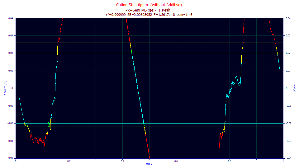
Although in this case the lack of normality is obvious, PeakLab does offer a stabilized normal probability (SNP) plot of the residuals with 90, 95, 99, and 99.9 % critical limits. For a density to be assumed normal to a 99.9% confidence, not one single pint should lie above the upper (or below the lower) red horizontal line. Clearly the normality assumption for the residuals fails.
We have just illustrated that the confidence and significance error statistics for the 1 ppm fit are not deemed statistically valid. And yet we have already shown that they catch incorrect or overspecified IRFs, and they catch incorrect, insufficient, and even close-to-overspecified core peak models.
One could argue that anything representing just 1 ppm of the data should never be analyzed at all, akin to studying six sigma outliers or attempting to compute a 99.999% confidence interval, but we have found the fit statistics at near zero error levels incredibly useful for screening models for correctness and the absence of overspecification. From a pragmatic perspective, we know a 95% confidence limit is not actually a true 95% band because of these assumptions being violated. At the same time, we do not dismiss the 1 ppm fit errors as having no value and nothing to tell us, much as we illustrated in the examples above. What we have chosen to do is strictly ad-hoc; we often use the 99% confidence statistics and simply assume they are probably closer to 90% confidence values.
It is also a practical consideration. For such exceptionally low error fits we could only conceive using bootstrap methods with a subsampling of data to estimate a more accurate error in fitting. Fourier methods require uniformly-spaced x-values. The fit we made of the above GenHVL<ge> data using Fourier methods required just .42 seconds for this 1400 point data set. To fit a non-uniformly sampled subset of this data as one element of a bootstrap, fitting the actual integral with an exceptionally fast quadrature routine, required 6.5 minutes. Since no bootstrap with a 95% level would be deemed valid without at least 1000 samples, this simple analysis would require 4.5 days. For a data set with many peaks, each of which would have to be independently fitted with the convolution integral, and to data sets of 10,000 or more points, a true error estimate might require a month or more of continuous computation.
We will also note that statisticians may not be your best source for validation the modeling within PeakLab. They may not see a goodness of fit near 1 ppm error as anything other than overfitting. It is altogether possible statisticians may go their entire careers, with an extensive experience in regression analysis, and never see data comparable to that which is observed in modern chromatographic instruments or models which so precisely describe real-world data.
The Concentration Test
The higher moment adjustments to the ZDD are amplified in the a3 chromatographic distortion operator which produces the observed fronting and tailing in the peaks. This makes the fitting of different concentrations a kind of litmus test for the robustness and universality of a chromatographic model. It must hold up at both dilute concentrations and at analytic concentrations where a small measure of overload slips in, as often occurs in practice, especially when the object of the analysis consists of lower area component peaks.
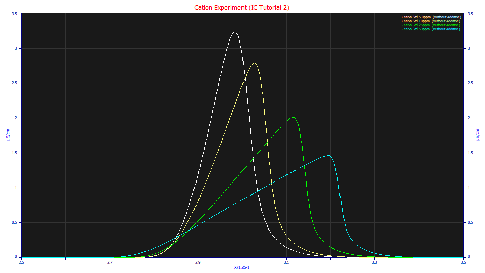
If we fit the GenHVL<ge> model to this standard peak at concentrations of 5, 10, 25, and 50 ppm, we would want the fits to be close to equally effective at all of these concentrations. These may seem small differences, but with respect to concentration-dependent shapes, in this case fronting, the differences are immense, as the area normalized plots of the data above suggest. Note that the 5 and 10 ppm (white, yellow) track one another in the initial rise, but the 25 ppm (green) deviates slightly, and the 50 ppm (blue) significantly, suggesting a small measure of overload in these two higher concentration samples.
If we fit these four data sets to the GenHVL<ge> model, we realize fits of 2.11, 1.46, 1.92, and 7.21 ppm error respectively. One would expect the fits to improve with concentration (because the S/N improves), but only to that point where a measure of overload starts to appear (since the once-generalized models do not process overload). We have four vastly distinct peak shapes, and only the last of these has a somewhat higher fit error. For a model to fit such highly differentiated fronted shapes, it must be capable of accurately representing the true ZDD since the a3 chromatographic operator translates this ZDD into these concentration dependent shapes. To fit this variation in shapes above, the ZDD model, and the estimation of the IRF, must be exceptionally accurate.
For example, the GenHVL[G]<ge> model, which uses the Skew Normal or GMG ZDD, and which performed so well with the 10 ppm data, realizes 1.86, 1.16, 5.63, and 124.8 ppm errors across these four concentrations. The model works well at low concentrations but not at higher ones.
If we look at the Gen2HVL<ge> twice-generalized model which adds a fourth moment adjustment to the once-generalized default chromatographic model, we see fits with 1.07, 1.36, 1.10, and 2.79 ppm error. This is exactly what a twice generalized model should do, the fourth moment adjustment managing the presence of this small amount of overload.
The Ideal Fit
Have we found the ideal fit? In the real world of statistical modeling, we doubt if any such entity exists. An ideal fit would account everything in the physical process, however small, and we know the PeakLab models cannot do this. No statistical model could do so.
Have we found a suitable universal model for analytic non-gradient shapes? We will leave that assessment to PeakLab's users. We will, however, note that we feel it likely that you will find the once generalized GenHVL and GenNLC models, and the twice-generalized Gen2HVL and Gen2NLC models, to be precisely this.
We must again note the absolute limitations of the nonlinear fitting process. A data set of all intrinsically tailed peaks is unlikely to fit the IRF accurately in an IRF-bearing model since the direction of each peak's native distortion will be the same as that of the IRF, and thus correlated to some measure. An ideal fit would process a set of intrinsically tailed peaks as effortlessly as a data set containing one or more intrinsically fronted peaks. The nature of the nonlinear fitting process makes that impossible. For such tailed peak data, the IRF must be independently estimated and then preprocessed using Fourier deconvolution in order to realize this same kind of effective fit.
The addition of a gradient, and of overload shapes, are managed quite well by the twice generalized models, but a better gradient fit is realized by first modeling and then unwinding the gradient prior to fitting, and the preparative shapes are better fit using an extension to the twice-generalized model that allows the two sides of the ZDD to have independent widths.
The PeakLab chromatographic models are based on a statistical generalization of the Haarhoff-VanderLinde and Wade-Thomas theoretical models. This generalization accounts multiple adsorption site and other asymmetry as well as the addition of two component IRFs that map nearly all of the distortions in a peak that are not a part of the actual chromatographic separation. In our view, these models are not merely built on sound science, but upon the very finest of that science.
While we may not have managed an absolute ideal, and while there may be more of a tool set of functions for this highest accuracy modeling as opposed to a single universal model, we have mathematically accounted nearly everything that can be fitted within the nonlinear modeling of chromatographic peaks. Much is new. You can now quantify the 'aggressiveness' of adsorption with the a4 third-moment parameter which is added to the core HVL and NLC models. You can quantify the narrow width and higher width components of the instrumental and system distortions, identifying differences in preps, run conditions, flow paths, and detectors. You will be able to quantity the changes in a column's performance with time. If you are designing columns, you will be able to quantify design changes in particles, particle treatments, pore sizes, materials, and transport.