PeakLab v2 Documentation Contents R2N Software Home R2N Software Support
Chromatographic Experiments (Tutorial)
For this tutorial, we will fit an extensive chromatographic experiment to study the impact of both concentration and additive level on the fitted peaks. Specifically, we want to see how the system variables of sample concentration and additive level impact the same six peaks in the cation standard we used in the first tutorial.
Importing the Data
![]() Click the Open button, the first button in the program's main toolbar. Select the file CationTutorial2.pfd
from the program's installed default data directory (\PeakLab\Data).
Click the Open button, the first button in the program's main toolbar. Select the file CationTutorial2.pfd
from the program's installed default data directory (\PeakLab\Data).
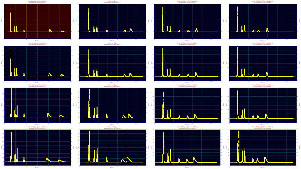
The sixteen data sets are contained in a single PeakLab PFD data file. This data have already been transformed for a retention or k' capacity factor scale and the baseline subtraction has been done. No IRF has been deconvolved. For this experiment, we will take the additional time to fit the IRF in each of the data sets. We want to know if the sample concentrations and additive levels alter the instrument response function, the IRF.
Visualizing the Effects of Concentration and Additive
Right click the second graph in the grid and choose Select as Principal Data Set from the popup menu. This data set will now have a red background. Click the Unselect All button in the dialog. All of the graphs except the principal data set will now have a gray background. Left click the the second graph in each of the three remaining rows to reselect these three data sets. The 6th, 10th, and 14th graphs will now have a blue background. Only the principal and selected graphs pass to the visualization procedure.
Click the View and Compare Data button.
For the Format, select Single Plot, for the Normalization select None, and for the Adjustments, leave Force Zmin=0 checked. Using the mouse, box the first set of peaks to zoom in this section of the data.
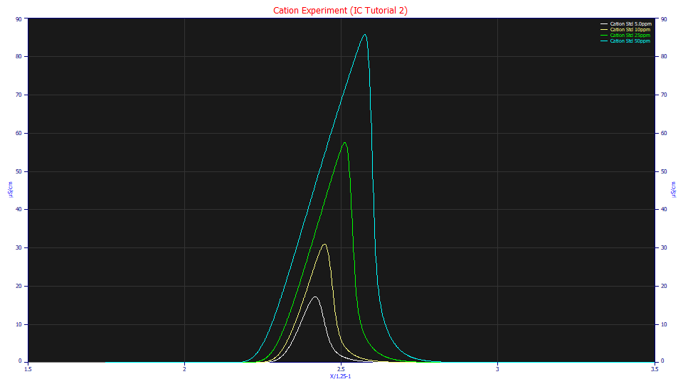
As the concentration increases, the first cation peak, Li+, becomes much more strongly fronted. This fronting or tailing is the chromatographic shape modeled so beautifully by the a3 parameter in the HVL, NLC, GenHVL, and GenNLC models. This a3 is a common chromatographic distortion to all of these models. When a3 is negative, a peak is said to be intrinsically fronted.
Right click the graph and select the Restore Scaling - Undo Zoom item from the popup menu. Zoom-in the last set of peaks.
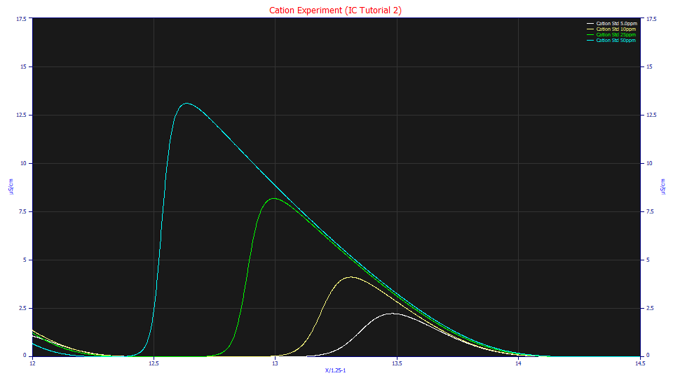
As the concentration increases, the last cation peak, the Mg+ cation in the standard, becomes much more strongly tailed. When a3 is positive, a peak is said to be intrinsically tailed.
Click OK to exit the Visualization procedure, and then click the Select All button in the main window. Click the View and Compare Data button.
Check Contour and Unit Area.
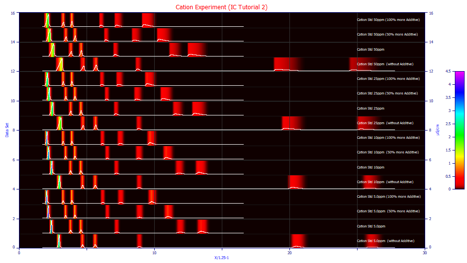
At each of the concentrations, the effect of additive level profoundly impacts retention. At a 2x additive level, the Mg+ peak elutes at a retention less than 10. When no additive is used, the retention of this peak occurs at a retention of 26.
Using the mouse, zoom-in the eight peaks to the right and then select the 3D Shaded option.
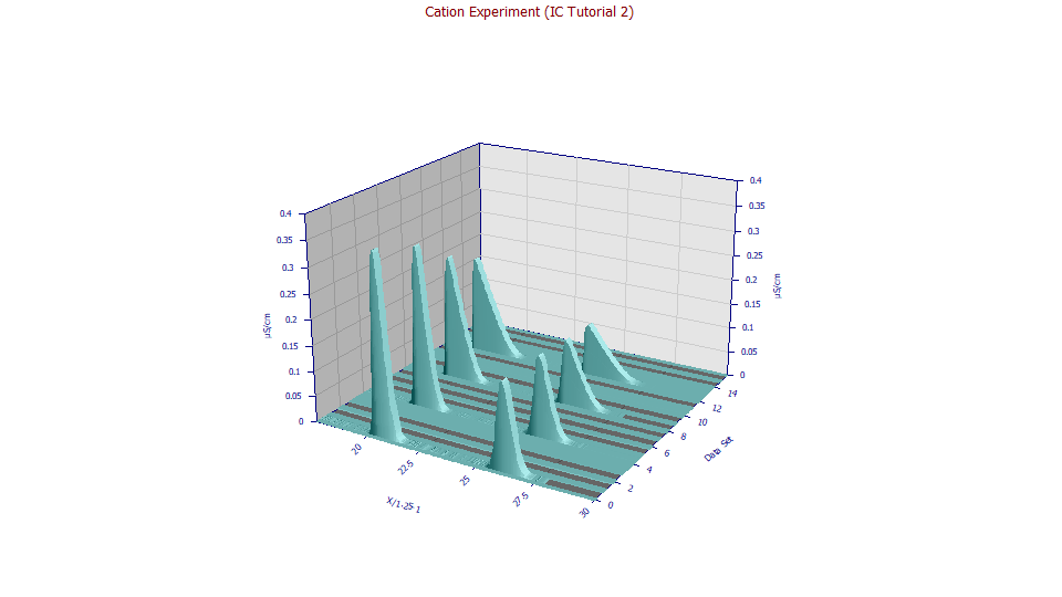
These are the Ca+ and Mg+ cation peaks for the zero additive case. The concentration will typically influence the peak shape more than any other factor. The additive clearly impacts location. To fully understand the differences, however, we will fit the data to a high level of accuracy.
Fitting the GenNLC<ge> Model
Click OK to exit the visualization procedure. Click the Local Maxima Peaks button. You will see the peak placement screen. Ensure the following settings are selected:
Peak Detection
Set Sm
n(1) to 25
Peak Type
Select Chromatography
in the first dropdown
Select GenNLC<ge> as the model in the
second dropdown
Scan
Set the Amp %
threshold to 1.5 %
Leave Use Baseline Segments unchecked
Be sure Use IRF,ZDD is checked
Vary
Leave width a2
and shape a3 checked, all other unchecked
You will note that each of the data sets has an automatic placement of this model with 6 peaks.
Click the IRF button. If you made modifications to the IRF defaults prior to this tutorial for your own fitting, please use the Save button to save your IRF values before resetting the defaults. Click the Defaults button. These are based on retention scale averages of modern IC data for each of the IRFs built into the program. Click OK.
We will fit the <ge> IRF, the narrow width component of the IRF a half-Gaussian which may better fit the axial dispersion.
Click the Peak Fit button in the lower left of the dialog to open the fit strategy dialog. Select the Fit with Reduced Data Prefit, Cycle Peaks, 2 Pass, Lock Shared Parameters on Pass 1. Be sure the Fit using Sequential Constraints box checked. Click OK.
If it is checked, uncheck the Iteration Update button to speed up fitting. This stops the graphical update with each iteration where an improvement in fit occurred.
Because we are fitting 16 data sets each with 6 peaks, we are fitting 96 convolution integrals with a high data sampling density. Even using all of the cores of your processor in a multithreaded fitting, these sixteen fits will require a couple of minutes.
Reviewing the Various Fits
Click Review Fit.
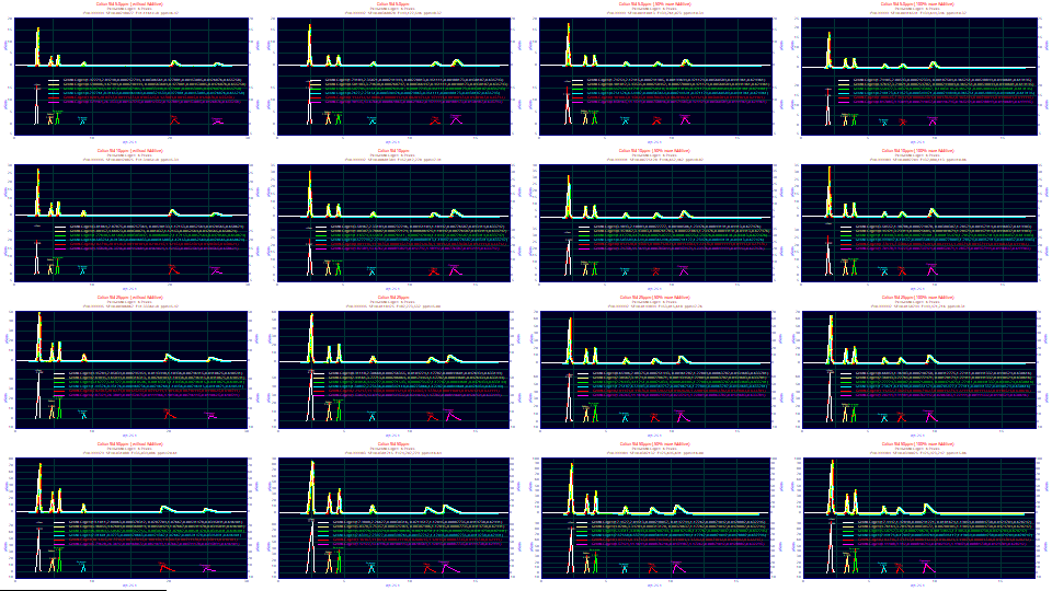
The fits range from 4.99 to 20.61 ppm unaccounted variance, superb goodness of fit given that six peaks were fitted rather than one, and the baselines were oscillating and prone to introducing error in the fitting.
Right click any graph and select Map Identifying Labels to Specific Peaks.
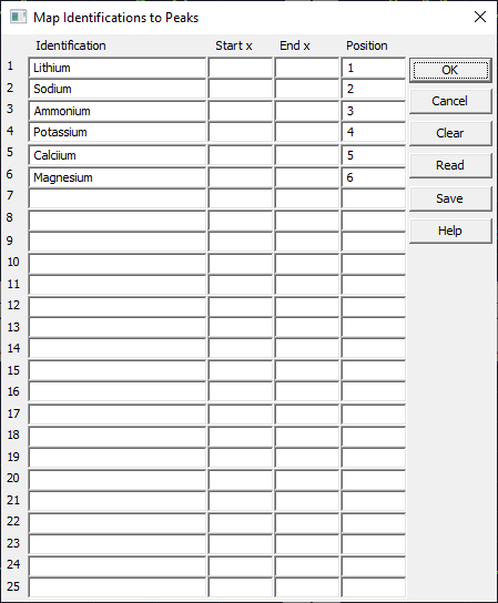
Use this option to label peaks in a chromatogram. These have already been added to the data file. The peaks are specified by sequential order since the x locations vary greatly with additive. Click OK.
Right click any graph and select Map Experimental Process Variables for Fitted Data Sets.
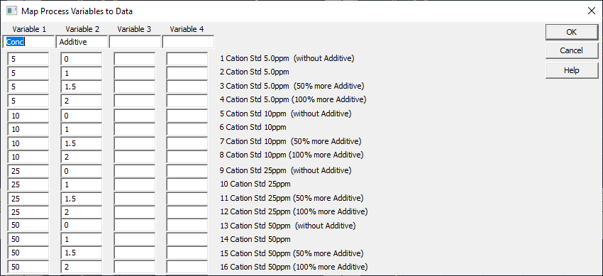
Use this option to specify numeric variables associated with an experiment. Here we specify the concentration (ppm) and additive level (as fraction of recommended amount). These have also been added to the data file. The titles are shown to help with entry. Click OK.
Click Numeric if the Numeric Summary is not displayed. In the Options menu first choose Select Only Fitted Parameters and then check Average Multiple Fits. Scroll to the bottom of the report.
Average�for�16�Fits
Fitted�Parameters
r2�Coef�Det�� DF�Adj�r2���� Fit�Std�Err�� F-value������ ppm�uVar
0.99998974��� 0.99998972��� 0.01494899��� 58,763,437��� 10.2583889
�Peak�� Type�������� ������a0���� ������a1���� ������a2���� ������a3���� ������a4���� ������a5���� ������a6���� ������a7����
����1�� GenNLC<ge>�� 8.07933699�� 2.30784582�� 0.00026474�� -0.0099790�� 1.11887780�� 0.00737138�� 0.04298459�� 0.63436801��
����2�� GenNLC<ge>�� 2.25247000�� 3.77100711�� 0.00029000�� -0.0016692�� 1.11887780�� 0.00737138�� 0.04298459�� 0.63436801��
����3�� GenNLC<ge>�� 2.61798274�� 4.54185798�� 0.00027606�� -0.0009040�� 1.11887780�� 0.00737138�� 0.04298459�� 0.63436801��
����4�� GenNLC<ge>�� 1.18633675�� 7.21994862�� 0.00039513�� 0.00189375�� 1.11887780�� 0.00737138�� 0.04298459�� 0.63436801��
����5�� GenNLC<ge>�� 2.52764231�� 12.3193707�� 0.00086418�� 0.01870488�� 1.11887780�� 0.00737138�� 0.04298459�� 0.63436801��
����6�� GenNLC<ge>�� 3.58747556�� 15.2877892�� 0.00099840�� 0.02611155�� 1.11887780�� 0.00737138�� 0.04298459�� 0.63436801��
CV�Percent�for�16�Fits
Fitted�Parameters
r2�Coef�Det�� DF�Adj�r2���� Fit�Std�Err�� F-value������ ppm�uVar
0.0004641%��� 0.0004651%��� 90.853670%��� 62.200140%��� 45.247606%
�Peak�� Type�������� ������a0���� ������a1���� ������a2���� ������a3���� ������a4���� ������a5���� ������a6���� ������a7����
����1�� GenNLC<ge>�� 80.621242%�� 15.246945%�� 15.044717%�� 82.950830%�� 10.605790%�� 24.030050%�� 3.0855039%�� 1.7568393%��
����2�� GenNLC<ge>�� 80.900316%�� 15.015629%�� 10.702513%�� 91.723675%�� 10.605790%�� 24.030050%�� 3.0855039%�� 1.7568393%��
����3�� GenNLC<ge>�� 80.982331%�� 15.015673%�� 10.937966%�� 112.55012%�� 10.605790%�� 24.030050%�� 3.0855039%�� 1.7568393%��
����4�� GenNLC<ge>�� 80.944661%�� 15.048280%�� 11.782047%�� 84.882322%�� 10.605790%�� 24.030050%�� 3.0855039%�� 1.7568393%��
����5�� GenNLC<ge>�� 100.77145%�� 43.246458%�� 26.962165%�� 134.35685%�� 10.605790%�� 24.030050%�� 3.0855039%�� 1.7568393%��
����6�� GenNLC<ge>�� 83.137941%�� 44.156155%�� 31.510942%�� 87.437350%�� 10.605790%�� 24.030050%�� 3.0855039%�� 1.7568393%��
The goodness of fit averages 10.2 ppm unaccounted variance and an F-statistic of nearly 59 million. If we look at the shared parameters held constant across the different peaks, we see the a4 ZDD asymmetry to be somewhat higher than the theoretical value for the NLC (1.11 instead of 0.5), and a CV% (SD/Mean) of 10.6%. This ZDD non-ideality doesn't vary a huge measure, but enough to give reasonable attention within the experiment. The <ge> IRF's half-Gaussian component, a5, much narrower in width (here an SD width), has a 24% CV. This we will give a fair attention in the experimental evaluation. The a6 exponential component of IRF is much wider (this is a time constant), responsible for most of the secondary tailing in the peaks, and with a 3.09% CV, very close to constant across the sixteen data sets. We can look for trends, but their impact will be small. The a7 parameter which specifies that 63.4% of the IRF is to consist of the Gaussian has an even narrower 1.76% CV. Again, we can look for trends, but we would expect little impact upon peak moments and properties.
Exploring the Parametric Relationships
Click Explore. Select 3D Shaded. Enter Conc for x in the first dropdown, Additive for the y in the second dropdown, and Parameters for the z in the third dropdown. Change the Peaks to view from Peak 1 to Peak 1- we will start with just the Lithium peak, the one most strongly fronted.
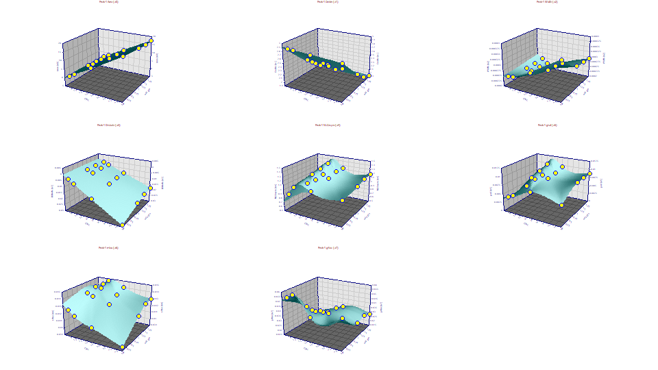
This is the visualization of the experiment. The concentration of the solutes in the standard is on the X-axis, and the additive level is on the Y-axis. The eight plots are for the GenNLC<ge> parameters a0-a7 for the first cation peak (Lithium). We will use this visualization to understand as many of the relationships of chromatographic modeling as we can.
a0 Area
Double click the first graph. This will produce a plot of just the Area. Select 3D Gradient.
If you have a wheel-mouse, spin the wheel forward and backward to rotate the surface by the angle in the XY plane. To change the Z angle, press the tilt wheel left or right. Click the wheel to restore the XY and Z angle settings before the changes were made.
![]() The Modify Graph View button in the graph's toolbar can also be used to adjust the different 3D
settings.
The Modify Graph View button in the graph's toolbar can also be used to adjust the different 3D
settings.
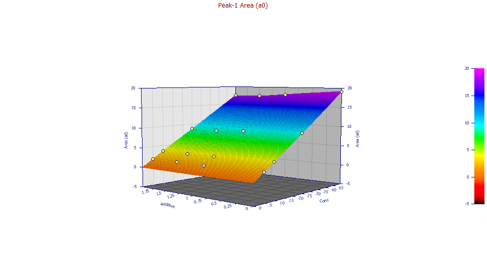
At the higher concentration, there is clear diminishing of retained solute with increasing additive. The colors in the gradient correspond with the Z area scaling. If you look closely at the colors, you will see some indication that there is also an effect of diminished peak area even at the lower concentrations.
Click 2D Contour. You are now looking straight down at the surface from above.
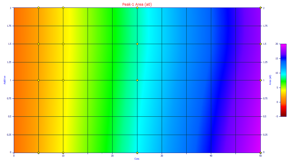
The impact of additive on the area of the peaks at the four different concentrations is now sharply visualized. The effect at the 25 and 50 ppm solute concentrations is clear. The effect at the two lower concentrations is less evident.
Using the mouse, zoom-in the contour by boxing just the lower concentration points.
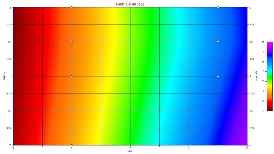
Here we are looking at a zone of the 3D interpolated surface formed from 16 points. One must be careful in reading too much into areas where no data is present. In this case, it is clear that even at low concentrations, the additive reduces the amount of the Lithium cation retained.
Right click the graph and select Restore Scaling - Undo Zoom or Custom Scaling from the popup menu. Double click the graph to restore all of the graphs.
a1 Center
In the GenNLC model, a1 is the deconvolved mean of the zero distortion density, in this case a generalized normal.
Double click the second graph.
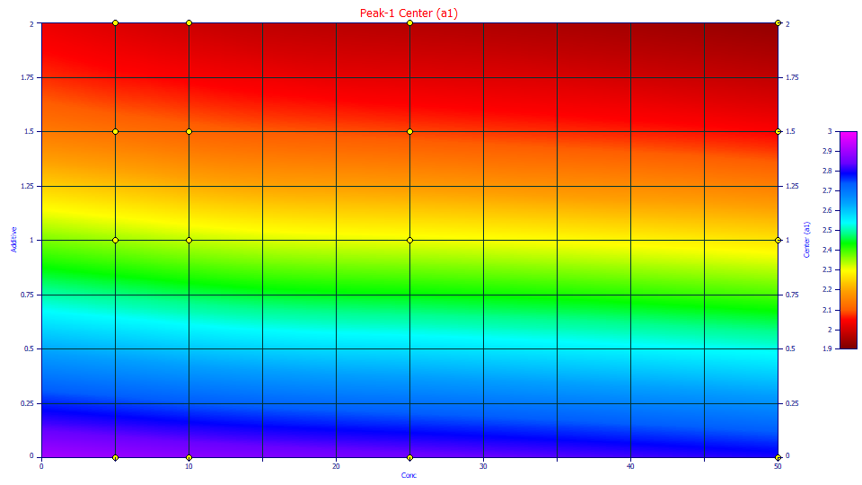
The contour illustrates the massive dependency of location upon the additive level. The greater the additive, the earlier the elution. The concentration also has a small impact. Higher concentrations elute slightly earlier.
Double click the graph to restore all plots.
a2 Width
For the GenNLC models, a2 is a first order time constant, the inverse of the rate in the Giddings density.
Select 3D Gradient. Double click the third graph.
If you have a wheel mouse, adjust the XY angle by spinning the wheel up and down to where the angle covers the shallow depression in the interpolated surface.
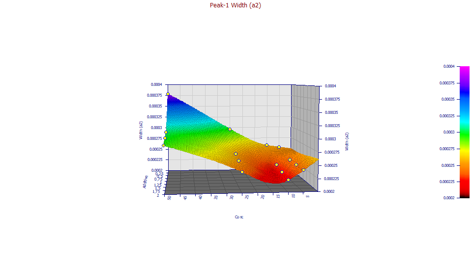
The angles chosen (XY=85, Z=5) show only modest increases with additive until the 50 ppm concentration (likely having a measure of overload) occurs. One would expect to see a consistent increase in width with concentration, not the well suggested by the interpolation.
Select 2D Contour.
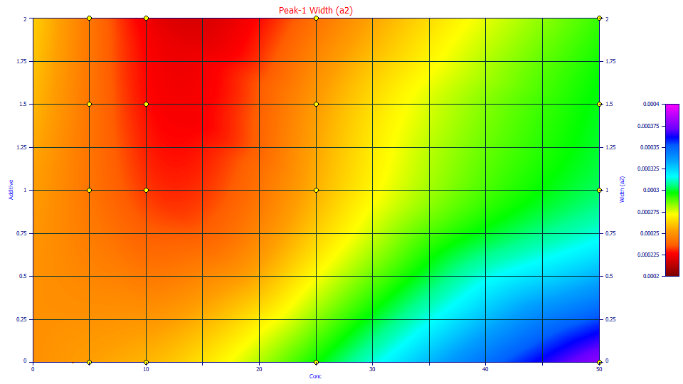
Here we see the three 10 ppm concentrations with additive comprising this valley or minimum in the response surface. It is likely real; the fitted a2 widths are actually smaller at 10 ppm on the additive samples. Without additive, the peaks elute later and have higher widths.
Double click the graph to restore all plots. Select 3D Gradient.
a3 Chromatographic Distortion
Double click the fourth graph.
![]() Click the Start/Stop 3D Animation button in the graph's toolbar to begin a 3D animation of the
surface.
Click the Start/Stop 3D Animation button in the graph's toolbar to begin a 3D animation of the
surface.
![]() If you have too fast or too slow an animation, you can adjust the angular increments and program in the
Modify
3D Animation Settings option.
If you have too fast or too slow an animation, you can adjust the angular increments and program in the
Modify
3D Animation Settings option.
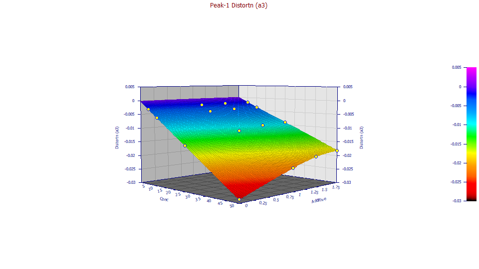
Note that overall relationship of the a3 intrinsic chromatographic distortion appears linear at each of the additive levels and the difference is mainly in the slope.
![]() Click the Start/Stop 3D Animation button in the graph's toolbar to stop the animation. Click 2D
Contour.
Click the Start/Stop 3D Animation button in the graph's toolbar to stop the animation. Click 2D
Contour.
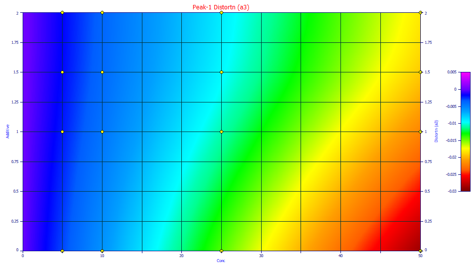
This is the parameter which addresses the unique skewness or third moment behavior which determines the principal fronting or tailing in a chromatographic shape. As you animated the 3D surface, you were animating the default 3D rendering, which is an interpolant. Any deviation will be seen in a lack of local planar shape in the rendered surface. The science behind the Haarhoff-VanderLinde and Wade-Thomas common chromatographic distortion is every bit as good as this a3 surface suggests.
We call the a3 parameter the "intrinsic" chromatographic distortion because it is the true shape, the true fronting or tailing, absent the IRF and absent the non-idealities in the underlying density. When you fit a GenNLC or GenHVL model, you deconvolve a true chromatographic shape, the one that would ideally exist for the given concentration of the solutes. Although the a3 distortion in the NLC and HVL models have very different theoretical derivations (one associated with the rate constants of adsorption and desorption, the other with the adsorption isotherm), the a3 distortion operator for both models produces identical chromatographic shapes for a given zero-distortion (infinite dilution) density. In fact, for the GenHVL and GenNLC, these were adjusted to be identical in value.
a4 ZDD Zero-Distortion Density Asymmetry
The parameters from a4-a7, the a4 ZDD asymmetry, and the a5-a7 IRF, are shared across all peaks. The next graphs will be identical irrespective of which peak is being inspected. Although these four parameters were shared, and increased the overall count of fitted parameters from 24 to 28, the difference in fit is immense. We will look closely at the ZDD and IRF parameters for any trends.
Double click the graph to restore all plots. Select 3D Gradient.
At this point note that the a4 and a5 plots show approximately the same overall shape of surface. In statistical terms, this means the parameters will be correlated and more difficult to fit with accuracy. Indeed, these are the two parameters with the least significance (the lowest absolute t-value in the Parameter Statistics in the Numeric Summary). We will keep this correlation in mind as we survey the relationships.
Double click the fifth graph.
![]() Click the Start/Stop 3D Animation button in the graph's toolbar to begin a 3D animation of the
surface. Click the left mouse button on the graph when the there is increasing concentration to
the right. This pauses the animation at the present position.
Click the Start/Stop 3D Animation button in the graph's toolbar to begin a 3D animation of the
surface. Click the left mouse button on the graph when the there is increasing concentration to
the right. This pauses the animation at the present position.
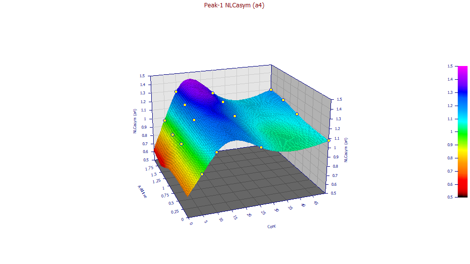
The fitted a4 ZDD asymmetry is far more sensitive to the concentration, increasing from 5 to 10 ppm, and then decreasing at 25 and further decreasing at 50 ppm. The obvious inference is that ZDD asymmetry is close to the theoretical (though still higher) at the lowest concentration, that such then increases, and that the subsequent decrease is perhaps associated with a small measure of overload. Since the additive only marginally impacts a4, we have close to four replicates at each concentration. This does suggest the asymmetry does have a concentration dependency. In all 16 fits, we are well above the 0.5 a4 theoretical asymmetry of the pure NLC and its Giddings zero-distortion density.
Click the left mouse button on the graph to restart the animation.
![]() Click the Start/Stop 3D Animation button to stop the animation. Double click the graph to
restore all plots.
Click the Start/Stop 3D Animation button to stop the animation. Double click the graph to
restore all plots.
a5 Fast IRF Component - Half Gaussian SD
Double click the sixth graph.
If you have a wheel-mouse, spin the mouse wheel to rotate the surface by the angle in the XY plane until you see increasing concentration, similar to the a4 plot.
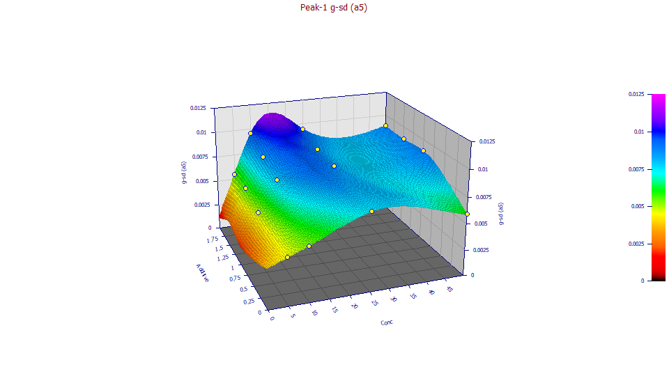
Unlike the prior plot, the a5 fast half-Gaussian component of the IRF, increases somewhat with increasing additive level. The values are narrow, the trend reasonably confirmed. This fast component of the IRF little impacts tailing, and is subtle, more difficult to fit. This was the parameter determined with least accuracy in the fitting, though still strongly significant with respect to statistical significance tests.
Double click the graph to restore all plots.
a6 Slow IRF Component - Exponential Time Constant
Double click the seventh graph.
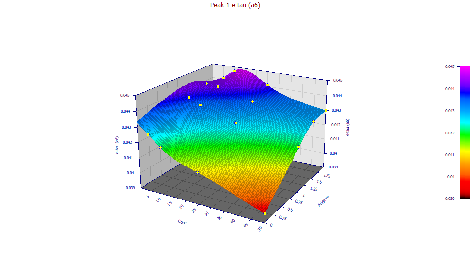
Amazingly, the exponential plots with a strong response surface despite only small differences in the a6 value across the sixteen different fits. The exponential width is impacted by concentration, decreasing with increasing concentration. The impact of additive, in general, is to increase the a6 tau.
Double click the graph to restore all plots.
a7 Half-Gaussian IRF Component Area Fraction
Double click the seventh graph.
If you have a wheel-mouse, spin the mouse wheel to rotate the surface by the angle in the XY plane until you see a similar surface to the one below:
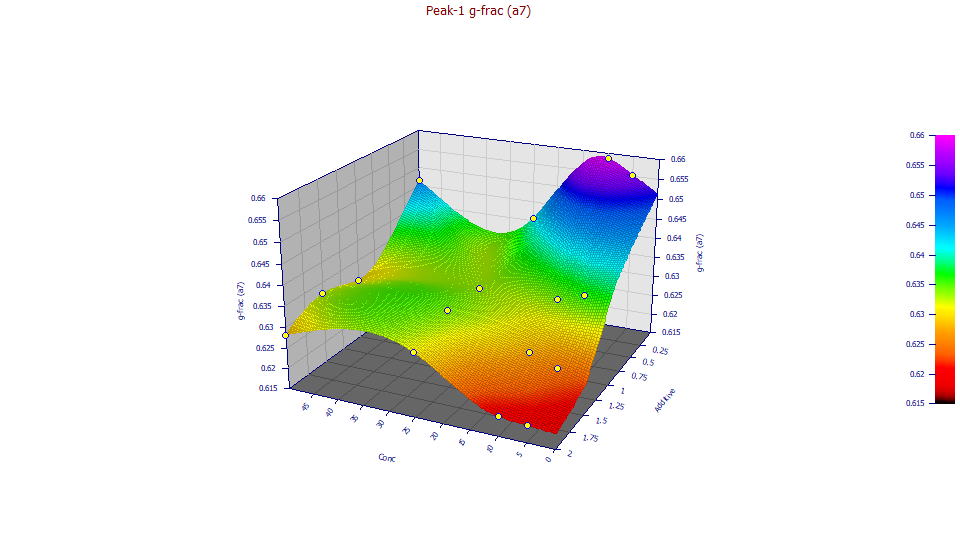
The half-Gaussian component of the IRF is important, fitting to better than half the area in the IRF. It is much narrower in width, however, and thus far less visible with respect to introduced tailing. The a7 half-Gaussian fraction decreases with additive, especially at lower concentrations. All of values are very close to the 5/8 half-Gaussian, 3/8 exponential assumption which was made in the first tutorial. At higher concentrations, the impact of additive is less pronounced. The relationship with concentration is less determinate.
Exploring the Deconvolved Moments
Moments as Fitted
Double click the graph to restore all plots. Change the z variable to Moments. If you have a wheel-mouse, spin the mouse wheel to rotate the surface by the angle in the XY plane until you see a respectable view of all five surfaces.
![]() If you do not have a wheel-mouse, click the Modify Graph View button in the graph's toolbar and
change the XY angle to 220 degrees, the Z angle to 20 degrees.
If you do not have a wheel-mouse, click the Modify Graph View button in the graph's toolbar and
change the XY angle to 220 degrees, the Z angle to 20 degrees.
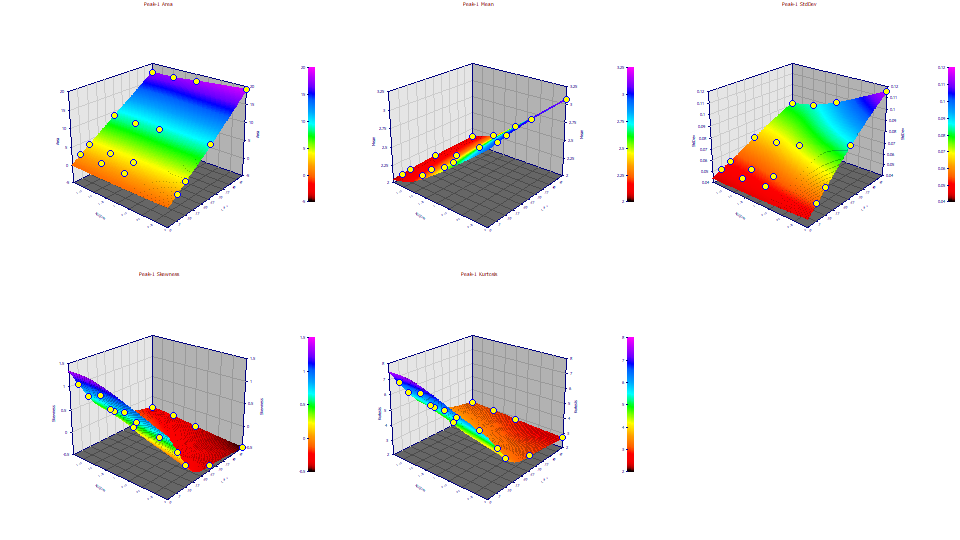
Unlike the parameter relationships, there is a consistent and clear defined surface for all of the moments. The third and fourth moments track one another since the predominate influence upon the thickness of the tails is the skew arising from the IRF. In the above surfaces, we are looking at the moments of the peaks as registered by the instrument. We will now take advantage of the deconvolution within the fitting to see the deconvolved moments. We will look at two levels of deconvolution, the peaks with the IRF removed, and the peaks with the IRF and ZDD removed. It is the latter that we deem most important. We continue to look at just the first peak of the six in the cation standard, the strongly fronted Lithium peak.
Moments with IRF Removed
Change the z variable to Moments DC1. This plots the moments for the first level of deconvolution, the GenNLC peaks with the IRF removed. We still see the intrinsic non-ideality within the chromatography, but we remove the instrumental/system distortion. To do this, we use the first five GenNLC<ge> fitted parameters in the GenNLC, the model with no IRF.
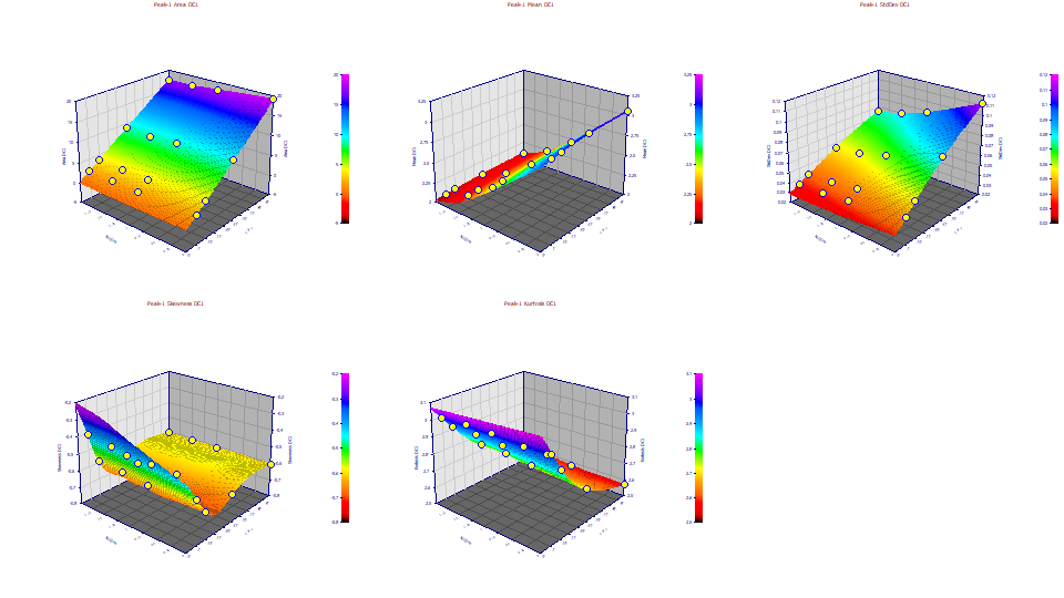
With the IRF removed, the third moment, the skewness, and the fourth moment, the kurtosis, look very different. For one, the skewness values are now all negative, indicative of the intrinsic fronting (left skew) for this first peak. The kurtosis now shows the tailing of the GenNLC thinning with concentration, so much so the kurtosis is well below the 3.0 of a Gaussian. On strongly fronted chromatographic peaks, the kurtosis can drop to such low values.
Moments with IRF and ZDD Removed - the Pure Chromatographic Peak
Change the z variable to Moments DC2. This plots the moments for the second level of deconvolution, the NLC peaks with both the IRF and the ZDD non-ideality removed:

Here we plot the pure NLC, the theoretical peaks with only the chromatographic a3 parameter impacting the higher moments. The IRF and ZDD deconvolution are implicit in the GenNLC<ge> fit. We only need to use the principal a0-a3 parameters to extract the pure NLC chromatographic peaks. Here we see the same <3 kurtosis as the concentration increases.
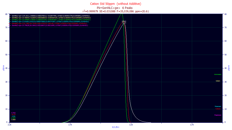
We will not do this as part of the tutorial, but if we were to select IRF Deconv. in the first dropdown of the main Review window, and Partial Deonconv. in the second, and zoom in the first peak in the first of the 50 ppm fits, we would see the GenNLC<ge> peak as fitted in the white curve, the GenNLC in the red, and the NLC in the green. Absent an IRF, a strongly fronted GenHVL, GenNLC, HVL, or NLC, can have an exceptionally sharp decay with a kurtosis well below 3.0. In general, however, the kurtosis of the deconvolved peaks will be very close to 3.0.
Smoothing Instead of Interpolating 3D Surfaces
Double click the Skewness plot, the fourth graph, in the Explore option.
![]() Click the Specify Surface Modeling button in the graph's toolbar. Select Fast Smooth and
C1 Smooth Surface. Set the Model Order to 2, and the Neighbor Count to 13. This produces
a locally smoothed quadratic surface instead of an interpolated one. For difficult relationships of parameters,
moments, and properties, you may need this local smoothing to visualize the trends.
Click the Specify Surface Modeling button in the graph's toolbar. Select Fast Smooth and
C1 Smooth Surface. Set the Model Order to 2, and the Neighbor Count to 13. This produces
a locally smoothed quadratic surface instead of an interpolated one. For difficult relationships of parameters,
moments, and properties, you may need this local smoothing to visualize the trends.
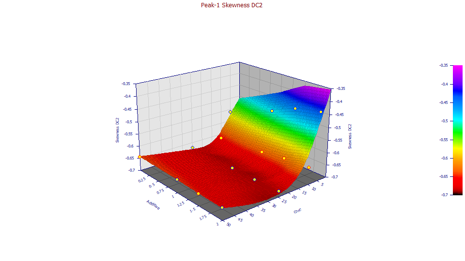
![]() When the points do not lie on the surface, you can click on the Modify Point Format in the graph toolbar
and select the Visible Only option. This will hide the points which would not be visible, those
hidden by the surface. This is particularly useful for animating smoothed surfaces.
When the points do not lie on the surface, you can click on the Modify Point Format in the graph toolbar
and select the Visible Only option. This will hide the points which would not be visible, those
hidden by the surface. This is particularly useful for animating smoothed surfaces.
Click Cancel. We will leave the surface as interpolant. Click OK in the the Explore Window to restore all graphs and click OK again to close the Explore option.
Click OK to close the Review window. Check Save updated information to the current data file when adding fits and click OK, accepting the default name for the fit. Click OK to confirm and click OK one last time to leave the placement screen and return to main screen.
In the third tutorial, we will subtract the average IRF from these fits from each of the data sets, and then fit a closed form model. We will see how much accuracy is lost when removing a system average IRF prior to fitting.