PeakLab v1 Documentation Contents AIST Software Home AIST Software Support
Understanding PeakLab's Chromatogtaphy Models
Spectroscopy and IRFs
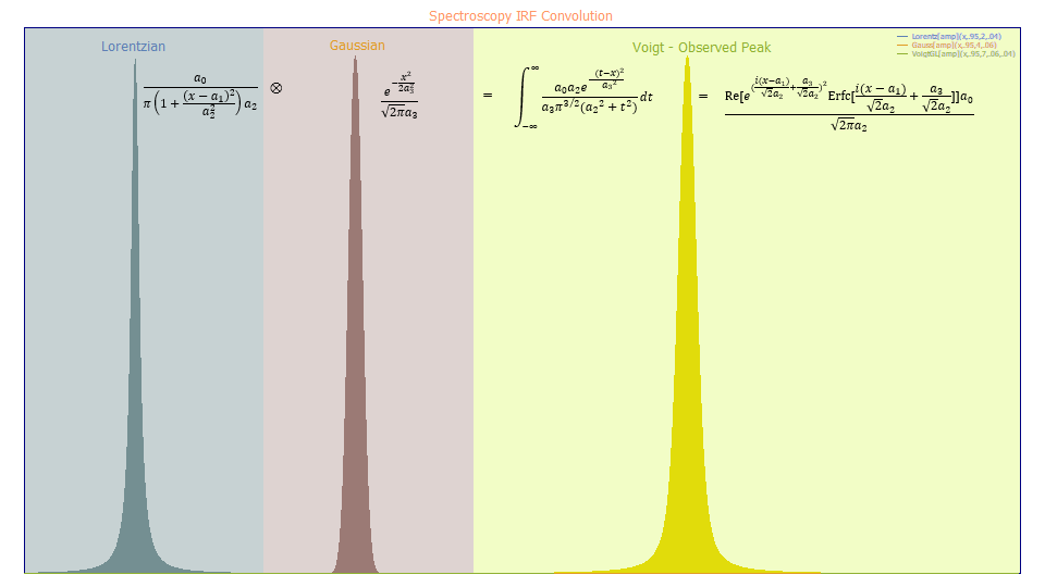
To understand the evolution of PeakLab's models we must begin with the real-world science we see well developed in the field of physics and in the system identification and transfer functions of the electrical engineers in the field of digital signal processing. The easiest way to understand IRFs, or instrument response functions, is to look at the true spectral line shape that is instrumentally observed in spectroscopy:

The natural spectral line is not a pure line, or delta signal, but rather a spectral line broadening that typically has a Lorentzian line shape. By spectral broadening theory, this shape arises from both natural and collision effects. It is worth noting that nonlinear modeling cannot discriminate multiple sources of Lorentzian broadening. The convolution of one Lorentzian with a second produces a Lorentzian whose width is the sum of the two.
In the real world, the true line shape, must be processed using an instrument whose optics will introduce a point spread function. The energy's frequencies will be further broadened by the lenses, mirrors, and other optical elements in the instrument as well as the optics and electronics in the detector. The combination of all of these added distortions is known as an IRF, the instrument response function. In general, the instrumental smearing in spectroscopy will be Gaussian.
To further complicate matters, Doppler broadening in spectroscopy arises from motions toward and away from an observer and is typically also Gaussian. Just as with two Lorentzian components, a Gaussian Doppler broadening and a Gaussian instrument response function cannot be separated from one another in a nonlinear peak fit. The convolution of a Gaussian with another Gaussian produces a third Gaussian whose width is the square root of the sum of the variances.
When a Lorentzian is convolved with a Gaussian, the resultant observed peak, as registered by the instrument, is a convolution integral whose shape is known as the Voigt model, a model whose tails will not decay as slowly as the Lorentzian, but not as fast as the much more compact Gaussian.
Decades ago, physicists developed pseudo-Voigt models (Voigt approximations) for this convolution integral. We will note that there is actually a Voigt closed form solution in the complex domain (shown above), but we can also note that two of the simplest density functions that exist in nature, the Normal (Gaussian) and the Cauchy (Lorentzian), do not combine in such a way to produce a real-domain closed form solution to this convolution integral. In other words, when one density is smeared by another of a different shape, things can get messy very, very quickly.
Chromatography and IRFs
The science of chromatography is appreciably more demanding in both the instance of the model for the true peak, that which arises from the chromatographic separation, and in the IRF which involves the distortions in a directional flow path. The following example uses actual parameters from real-world chromatographic data fits:
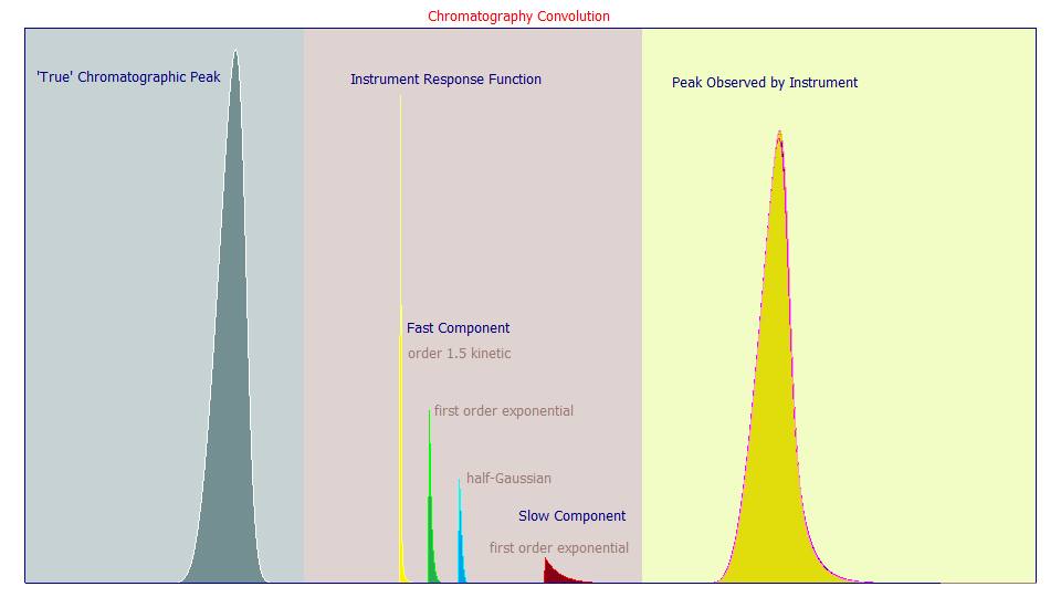
For the moment, we will set aside the issue of the true peak model, and look only at the non-chromatographic separation portion of the distortion, the IRF or instrument response function. From the perspective of that which can be successfully fitted, there will be both a narrow-width and a high-width IRF component. These will be one-sided, as all IRF distortions represent delays in the transport or measurement of the solutes. The IRF in a chromatographic convolution model will consist of the sum of two discrete (independent) distortions or delays.
In the above plot, the IRF curves are yellow, green, blue, and red, and each has the same area. If you look at the "true peak" on the left, and then the high width first order exponential IRF (the red IRF component), and finally the observed shapes on the right, you will see that most of the tailing in the observed peak comes from this high-width red component. We have never observed anything other than a first order kinetic model as appropriate for this higher-width IRF component, and we have found this wider IRF component, for a given instrument and column, to be largely constant; nearly independent of the prep, additives, temperature, and solute concentrations.
It is with the narrow IRF component where much gets muddled. We believe the axial dispersion is likely best represented by a one-sided, directional, half-Gaussian (the blue IRF component). The interphase mass transfer associated with porous media has a second order component where the overall resistances can be somewhat approximated by an order 1.5 kinetic decay (the yellow IRF component). One can also use a first order exponential for the narrow width component (the green IRF component) as an approximation for both effects (the half-Gaussian decay shape is close to a .5-.6 order kinetic decay). The good news is that the narrow width component has only a small effect on the overall peak shape and the three models can be used close to interchangeably. In the above plot, the peaks from each of the three narrow width IRF components almost completely overlay one another in the three observed peaks. The less than good news is that statistically one cannot achieve fit significance with more than one of these narrow width models in the overall IRF. Although we have found this narrow IRF component to be somewhat dependent on the prep, additives, temperature, solute concentrations, and retention, because its influence is small on the overall shape, it can generally be treated as common to all peaks in a chromatogram, and often across a wide range of samples and system variables.
One can thus treat the narrow width instrumental distortions as all half-Gaussian based axial dispersion, or all interphase mass-transfer resistances in a 1.5 order kinetic, or in a simplification where all narrow width distortions are also treated as a first order kinetic delay. Each will give an estimate of the quantity of this narrow width distortion and an estimate of the width, but non-linear fitting cannot include and separately quantify all of these different low-width effects. Statistically, the half-Gaussian is easiest to fit in the iterative non-linear fitting, the 1.5 order kinetic the hardest.
Note that the closest traditional chromatographic modeling has come to the above design is for the true peak to be treated as Gaussian, the IRF to be a single first order exponential, as in the red curve above, and the final peak to be an EMG. Such modeling, however widely used historically, will be of dubious value in modern chromatography. We have never observed the true peak to be a Gaussian, or the IRF to be a single exponential, in any real-world chromatographic data set.
The modeling problem is a challenging one. Fitting the IRF convolution integrals directly is far too slow; PeakLab's non-linear fitting is done in the Fourier domain.
Gradient HPLC Chromatography and IRFs
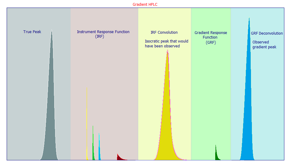
To make just the IRF portion of the modeling even more complicated, consider the addition of a deconvolution step after the final peak in the plot above. In this step, the isocratic peak that would be observed by the instrument is replaced by a deconvolution which cancels a measure of the right-side tailing distortion introduced by the IRF above. In this case, the HPLC gradient cancels out much of the influence of the IRF, while also dramatically compacting the tails of the observed peak. We have found an HPLC gradient to be well-modeled by a half-Gaussian deconvolution. Given that much of the isocratic IRF tailing arises from the higher width first order kinetic, there is no true cancellation, merely an additional alteration, a further complication, to the observed peak arising from this deconvolution describing the gradient compression of the peak shape.
The Generalized HVL Chromatographic Model
In the spectroscopy example, the IRF was a simple two-sided Gaussian, and even there, with two of the simplest densities that exist in nature, the convolution integral did not have a real-domain closed-form solution. For chromatographic peaks, the IRF is appreciably more complicated than a simple Gaussian. Further, the other component of the convolution, the "true peak", is vastly more complicated than a simple Lorentzian. There are no closed-form solutions to the convolution integrals of the real world chromatographic IRFs and the real world models which describe the chromatographic separation.
At this point, we address the 'true peak', the model describing the theoretical chromatographic shape, the fronting or tailing which increases with increasing concentration of the solutes. We begin with the similarity of the NLC and HVL models. It turns out the mathematics describing the tailing or fronting which occurs in a chromatographic separation is identical for the HVL model, a GC model derived using adsorption isotherm arguments (where a diffusion width is assumed Gaussian at infinite dilution), and for the NLC model, a non-linear LC model derived using first order kinetics of adsorption (where the width is assumed to follow the Giddings first-order kinetics at infinite dilution). In effect, despite immense differences in history, derivation, and parameterization, the two models are identical when the PDF and CDF (the zero distortion density and cumulative) are generalized.
The HVL math for a diffusion-based model can exactly replicate the NLC kinetic model shape, if the Gaussian ZDD (zero-distortion density) is replaced with the Giddings density. Similarly, the NLC distortion math can exactly replicate the HVL shape by replacing the Giddings ZDD with a Gaussian. The HVL and NLC models are strikingly similar because the Gaussian and Giddings densities are quite similar; the Gaussian is symmetric and the Giddings is almost a Gaussian shape except for a very slight right-shifted symmetry.
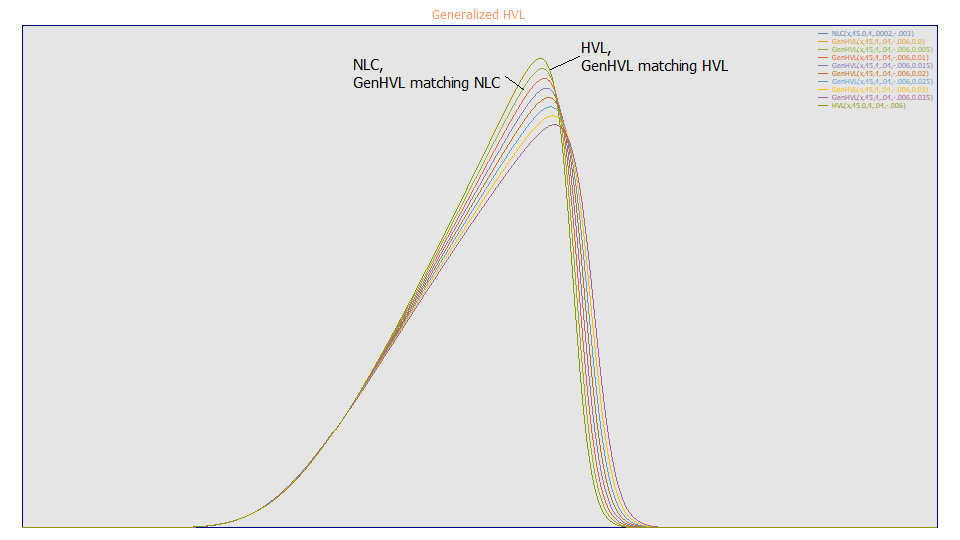
We must now leave the field of ChE and enter the field of the statistical sciences in generalizing a diffusion model for chromatography we call the generalized HVL, or the GenHVL. To build a generalized HVL, we replaced the Gaussian density with a generalized statistical density capable of modeling both the Gaussian and Giddings densities. PeakLab offers a wide choice of statistical ZDD densities. For the default chromatographic model with a statistical width, the GenHVL, we chose a generalized normal that was capable of reproducing the NLC to a much greater precision than the data can be collected, as well as a density which successfully modeled real-world data where the skewness in the infinite dilution density was almost always greater than that of the Giddings density.
The Generalized NLC Chromatographic Model
Since we discovered the pure HVL and NLC models have a common chromatographic distortion and shapes which vary only with an assumption of the ZDD, the zero-distortion or density observed at infinite dilution, it was a straightforward matter to create an identical generalized chromatographic model with kinetic arguments. This is the generalized NLC, the GenNLC.
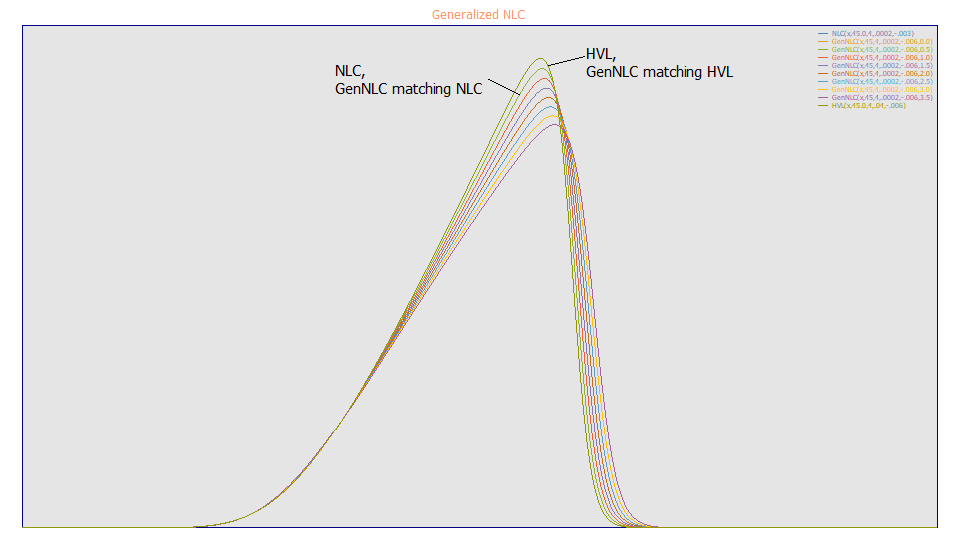
The GenHVL and GenNLC produce identical shapes, but differ in the parameterization. The GenHVL has a statistical width and a statistical ZDD asymmetry. The GenNLC has a kinetic width, as a first order time constant, and a ZDD asymmetry indexed to the NLC at a value of 1/2.
The GenHVL and GenNLC models can be used interchangeably, and in fact, the PeakLab Numeric Summary offers the option of displaying the equivalent parameters from the two different models. You can see both the NLC kinetic parameters and HVL diffusion parameters as part of an output from a given fit of either model.
The 'True Peak'
This is where we diverge once more into the domain of the signal scientists.
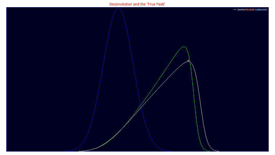
In the deconvolution plot above, the GenHVL is the white curve. The green curve is the pure HVL. The blue curve is the infinite dilution Gaussian that produces the green HVL when the chromatographic distortion operator is applied.
Which is the 'true peak'? In spectroscopy, there is no separation possible in the two Lorentzian components that give rise to the broadening. In chromatography, it is a matter of choice. The 'true peak' will almost certainly involve the removal of the IRF. If you also wish to see the pure HVL (or NLC), you choose one more level of deconvolution, the green curve. If you want to take the concentration of the solutes wholly out of the picture, you use the blue curve, the Gaussian (or Giddings). You can use whichever level of deconvolution is most applicable to your work. Each will have an identical area.
Why is Fitting Chromatographic Data So Difficult?
The simple answer is that the models that effectively fit nearly all of the variance in chromatography data to full statistical significance typically require the fitting of a convolution integral for each peak. The following is the formula for the simplest of the PeakLab generalized chromatographic models with an effective IRF, the GenHVL[Z]<ge>:

If you have a data set with a dozen different peaks, you will be fitting the sum of twelve of the above integrals to the data. Certain of these parameters will be shared across the different peaks, and others will be distinct to each peak. Further, unless the models, which have no closed form solution, are fitted in the Fourier domain, a single fit could easily require an overnight computation, or worse. PeakLab will manage such fits in a few minutes. Once the IRF is known and presubtracted using Fourier methods, the fits will be closed-form and require just a few seconds.
To manage such fits effectively, modern computer science programming techniques are used to simultaneously process the different convolution integrals. On the newer i9 eight core machines, PeakLab can process sixteen peaks simultaneously in the fitting. There is also the challenge of the algorithmic science, to ensure an iterative convergence to the true global solution. PeakLab may seam together as many as hundred or more individual fits to realize the optimal solution.


 |