PeakLab v1 Documentation Contents AIST Software Home AIST Software Support
Interpolate/Upsample
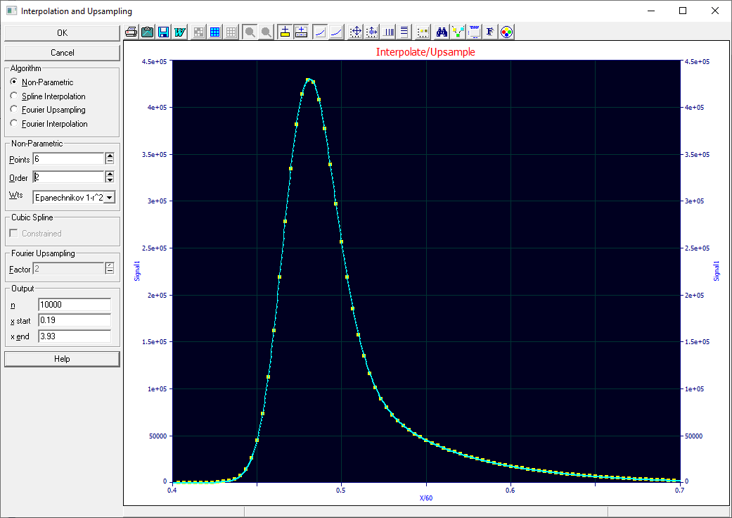
This option offers a very effective way to decrease or increase the size of the data table with minimally distorting the peaks within the data.

Non-Parametric Algorithm
The PeakLab Non-Parametric procedure is about the most advanced fitting algorithm you will find for fitting and smoothing data to create uniformly spaced and smoothed data of any sampling density from an existing data set. You have a choice of the points within the fit window, the order of the polynomial, and the weighting function. This is an extension to the Loess algorithm which offers a linear model and the tricube weighting function. The incoming data need not be uniformly spaced.
This is the only algorithm in this Interpolate/Upsample procedure that will also smooth the data.
Points
The higher the window point count, the greater the smoothing that will occur with the fitting. To avoid attenuation, you will probably need to fit at least a quadratic. If the data are noisy, you may need to increase this point count, and thus the smoothing, to avoid oscillations in the local model.
Order
Although this procedure is based on one whose origins used a linear model, you will probably want to increase the point count and use a higher order to avoid attenuation of sharp peaks. The cubic accuracy is an ideal of sorts for statisticians, and with the proper choice of a point count and weighting function, you may be able to successfully fit a cubic.
Weighting Function
We have arranged the weighting functions (after the first entry with uniform or equal weights - listed as 'no weighting') in order of the power of the weighting function. It is probably best if you simply experiment and find the weighting function that gives you the most stable fit. These come from a very different research work we did some years ago where that which we called 'TQ5' weighting, (1-abs(r)^3.5)^5, outperformed most of the other weighting models. If you are having difficulty getting stable fits with the cubic, try the TQ5 weighting before reverting to the quadratic or linear model.
With this Non-Parametric procedure, there are no bounds on the estimations. You can pick any starting x and ending x within the data range and you can specify any count of points in the output stream.
Spline Interpolation Algorithm
Both a standard and a constrained cubic spline are offered. The Constrained algorithm will reduce the order when the spline unstably rises above or below the band of points used for the estimate (the oscillations often seen between points in cubic splines). These splines are pure interpolants; there is no smoothing.
With this Spline Interpolation procedure, there are similarly no bounds on the estimations. You can again pick any starting x and ending x within the data range and you can specify any count of points in the output stream.
Fourier Upsampling
This can be an an exceptionally accurate and fast interpolation if you are willing to accept a multiple of the current data count. A Factor of 10 upsample on a 500 point data set produces a 5000 point data set with the same x-bounds. For a Fourier Upsampling to work well, the start and end of the data must decay to a strong zero baseline.
The Fourier Upsampling has no specification of output point count, although you can limit the output values to a specified range.
Fourier Interpolation
Because a Fourier transform is based on a set of continuous sines with coefficients, those can be used to reconstruct any density or range of x values in the data, albeit slowly.
The Fourier Interpolation procedure has no algorithmic adjustments.
You can select any starting x and ending x within the data range and you can specify any count of points in the output stream.
Final Data Count
You may set any number of points for the output data, up to a maximum of 1,048,576. The output set will have the same initial and final X values, and will consist of an equidistant X spacing. Within reason, you can thus reduce a data set to a smaller size while preserving the quality of the input data stream. You can conversely augment a data set with too few sampled points.
Data with Deleted Artifacts, Disabled Points, or Non-Uniform X Spacing
The equal X-spacing of the output data stream is important if you find it necessary to delete artifacts from a spectrum or chromatogram. The loss of a constant X-spacing seriously hampers or altogether ruins the effectiveness of a number of PeakLab's processing options. For example, all FFT based procedures are likely to suffer badly. This includes the FFT smoothing, Gaussian convolution smoothing, Fourier Domain Filtering, the IRF Deconvolution. Similarly, the Savitzky-Golay smoothing requires uniformly spaced X values. It is central to the AutoFit procedure based upon second derivatives.
While it is possible to effectively fit data with unequal X spacing using the AutoFit procedure based upon residuals in conjunction with the Loess smoothing procedure, you will probably be much happier if you simply use this non-parametric estimation to produce a uniformly spaced data set.
Window Point Count
The default window of 4 data points incurs the minimum of peak amplitude attenuation. Higher window counts, however, can be used to smooth the data. The power of smoothing will be roughly comparable to the Loess procedure.
Because of degree-of-freedom considerations, we recommend a minimum data window of 5 points with the quadratic model. If you encounter one or more points which clearly lie outside the data when using a quadratic model with a 4 point data window, you should increase the data window to 5 points.
Model
You have a choice of fitting either a linear, quadratic, or cubic model. For peak type data, the cubic or quadratic model are probably the better choices. They tend to produce less peak amplitude attenuation, and for a given window point count, less smoothing as well.
Real-Time Graphical Update
As you adjust the final data count, window size, or model, you will see a PeakLab Graph where the new points appear in reference to the original data . This enables you to effectively judge the density of the final data as well as any distortion of peak features occurring at higher window counts. Simply select OK to accept the modified data or Cancel to retain the original data.