PeakLab v1 Documentation Contents AIST Software Home AIST Software Support
GLM Performance Analysis
The Fit Performance button in the GLM Review opens a performance optimization set of plots to aid in choosing an optimum predictor count for GLM model fits.

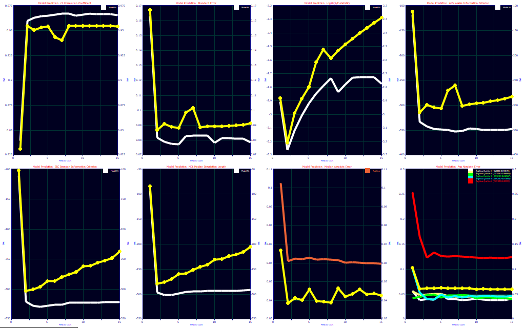
There are eight plots in the series. All of the prediction plots will be based on the type of Prediction Errors selected at the time of fitting. The performance metric is on the Y-axis and the count of predictors is on the X-axis. With the exception of the median and average error graphs, the last two in the second row, there is a reference curve containing the model fit (estimation, calibration) performance. This is a reference which can be toggled off and on using the button in the graph's toolbar.
Fit Performance Statistics
For the fit predictive performance statistics, the goodness of fit are described in detail in the GLM Numeric option. We will briefly summarize the eight in the performance plots.
N = count of data observations
np = count of parameters (includes constant)
nx = count of x predictors (np-1)
DOF = degree of freedom, N-np
SSE = sum of squared errors from the prediction
SSM = sum of squares about the mean of the dependent variable
MSR = mean square regression
MSE = mean square error
Log[] = natural logarithm
r˛ of Prediction
SE (Fit Standard Error)
F-stat (F-statistic)
AICc (Akaike Information Criterion corrected)
BIC (Bayesian Information Criterion)
MDL (Minimum Description Length)
Median Error
This is the median of all predicted values.
Average Error
This is the average of all predicted values. Average errors are also computed for the five quintiles of Y data.
In the above equations, SSE is the sum of the squared errors of prediction. If the Leave One Out method of Prediction Errors specified in the original fitting, there will be N separate fits, each with one of the N samples omitted The one omitted set is then evaluated to get a single prediction error for that sample. The sum of squared errors in these N predictions is the SSE. The SSM includes all of the Y values as all of the samples are represented.
If the Random Sampling method is specified, there will be a random count of prediction errors for each sample, one prediction error for each time that sample appears in an out-of-sample random set. That count may be zero for a given sample if the count of repetitions is too small and that sample never appears in an out-of-sample set. When the sample appears more than once, the prediction error for that sample will either be the average or the worst (highest error) value. If the random sampling is sufficiently specified, there will be a prediction error for each of the samples and the SSE and SSM will function similarly to the Leave One Out method. The difference is that the in-sample set fits will reflect the absence of the out-of-sample spectra. If the bracketing of the modeling problem has little redundancy, the loss of those out-of-sample spectra in the modeling can be appreciable and there may be large differences between the Leave One Out and Random Sampling prediction errors.
Plot 1: r2 Prediction
The first plot consists of the r2 of prediction. The sum of squares of the individuals errors, whether by Leave One Out or by average or worst case Random Sampling will be normalized by the sum of squares about the mean of the Y-data. This is the only plot of the eight where the optimum is at a maximum. In all others, the optimum will occur at the minimum.
Plot 2: Standard Error of Prediction
The second plot contains the predicted standard errors. The SE is the least robust estimate of prediction error since the error estimates are strongly influenced by outliers (high error predictions).
Plot 3: Log10(1/F-statistic)
To keep all of the performance criteria consistent, the F-statistic is plotted as the base-10 logarithm of the F-statistic inverse. This is shown in the third plot. This allows the F-statistic optimum to occur at the minimum instead of the maximum.
Plot 4 : AIC - Akaike Information Criterion (corrected)
The AICc, the corrected Akaike Information Criterion, is shown in the fourth plot.
Plot 5 : BIC - Bayesian Information Criterion (Schwarz)
The BIC, the Bayesian or Schwarz Information Criterion, is shown in the fifth plot.
Plot 6 : MDL - Minimum Description Length
The MDL, the Minimum Description Length is also a theoretical information criterion. The MDL is shown in the sixth plot.
Plot 7 : Median Error
The median error plot is a highly robust estimate of prediction error that is not influenced by large outliers or high error predictions. The median error is shown in the seventh plot. The reference in this plot consists of the average error (also shown as the main item in the eighth plot). The median error will almost always be smaller than the average error.
Plot 8: Average Error
The average error plot is a robust estimate of error that is less influenced by large outliers or high error predictions than the standard errors which uses the sum of the squared errors. The average errors are shown in the eighth and final plot. The references in this plot will consist of the average errors for the 5 different quintiles of Y values. You will often see the errors increase with the magnitude of the Y-values.
Optimization Average Count
For the optimization, you can choose to plot only the Best performing model for a given predictor count, or the average of 3, 5, 10, or 20 of the retained models. The plotted values will revert to zero if there are insufficient models of the specified count to generate an average.