PeakLab v1 Documentation Contents AIST Software Home AIST Software Support
IRF Concepts
Instrument Response Functions
In order to properly model chromatographic peaks, even with modern instruments, distortions arising from instrumental effects are generally best removed before the fitting occurs, or modeled directly in the fitting. In PeakLab, an instrument response function, or IRF, is the mathematical model describing these instrumental distortions. The reasoning is straightforward. In order to derive meaningful theoretical estimates of diffusion or kinetic coefficients, chromatographic distortion as a function of concentration, or other peak properties such as accurate moments, we want to estimate the true peak; not the peak plus instrumental artifacts.
As detectors and columns have advanced, the IRF distortions have lessened. They have not, however, disappeared. For example, there will always be mixing effects at the inlet and in the volume of a detector's chamber, which contribute to band broadening. There are the nonidealities from the lack of a pure laminar flow everywhere in the elution path. There is, in liquid chromatography, the axial dispersion which occurs throughout the flow path, contributing its own distinct form of band broadening. In general, IRF effects occur independent of the actual chromatographic separation, from system-wide distortions.
In PeakLab, such distortions are generally treated as constant across the peaks within a chromatogram, and can often be treated as constant across concentration differences of solutes, across temperatures, and in differences in the prep, including significant variations in additives. In some instances, they may be constant across preps and columns.
We have almost universally found that the IRF for chromatographic peaks must consist of two components, a higher width component almost always modeled with a first order kinetic decay (exponential), and a narrow width component that can be fitted as a one-sided probabilisitic component (half-Gaussian), or as a faster kinetic (order 1 or even 1.5).
We have observed an astonishing constancy with the higher width kinetic effects. Most variation will likely rest with the narrower width contributions to the distortion, and if these arise from axial dispersion, one would expect to see a measure of concentration dependence. In our experience, even that is modest across a considerable range of solute concentrations.
An IRF can be determined with accuracy only by fitting peak+IRF composite or convolution models. In PeakLab such composite models are represented similarly to "GenHVL<irf>", a generalized HVL convolved with irf, the specific IRF model. You will need to fit a reference or standard peak to such a composite model to determine with high precision the actual instrumental broadening.
Although this is one of the more challenging aspects of peak modeling, it is a well-established science (transfer functions, system identification), and it has a lovely payback in analytical benefits. For example, consider the following fit results from three different fits to data from a standard consisting of six IC peaks:
Fitting Model F-statistic r� ppm UnaccountedVariance
Baseline-corrected data GenHVL 130,000 0.996500 3500.0
Baseline-corrected data GenHVL<ge> 47,000,000 0.999991 8.7
<ge>Predeconvolved data GenHVL 7,500,000 0.999939 61.3
This is typical of what you can expect with IRF processing. Unless a fit fails to converge to the global minimum, there will be a dramatic improvement in the fitting when an appropriate IRF is fitted. For far faster processing times, it is of benefit to deconvolve the IRF prior to fitting. Since one is using a historical or predetermined estimate of the IRF's parameters, and since the deconvolution procedure increases the noise in the data, a fit to pre-deconvolved data will never be as good as the full composite model fit. Still, one sees most of the benefits, and such fits require seconds rather than minutes.
How Important is the IRF in Chromatographic Modeling?
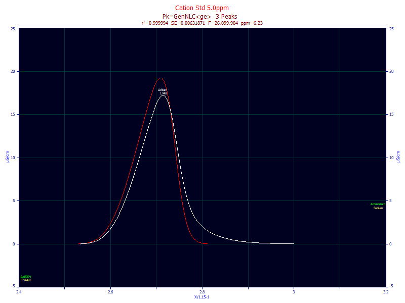
With respect to achieving the most accurate estimates of the different chromatographic properties of peaks, it is essential. Consider the following IC analytic peak from a standard with an exceptional S/N:

The white curve is the peak from the instrument; the red curve is the peak after the instrument's contribution to the shape has been removed by fitting. The difference can be this significant or even more so (this is an example of very modest instrumental distortion). Even at the routine concentration used for this standard, this peak, which is clearly fronted in its deconvolved shape, is somewhat ambiguous in its shape as measured by the instrument.
If possible, you should remove (deconvolve) the instrumental distortion of your data in one of two ways:
1. Once the IRF parameters for a given instrument/column/analysis have been identified, use Fourier deconvolution with an accurate Fourier domain filtering to remove the instrumental distortion from the data in a preprocessing step. The peaks are then fitted with non-integral (closed-form) models where the instrumental effects cease to be an issue. This generally requires only a S/N thresholding for the Fourier filter, and even that step can be automatic or even omitted if the data are of an exceptional quality and the IRF is an accurate representation of the instrumental broadening.
2. Fit a composite peak+IRF model to multiple peaks, sharing the IRF parameters across all peaks. This will usually be needed to initially determine the parameters of an IRF to a good accuracy. Once a given IRF has been predetermined, PeakLab makes it an easy matter to lock these IRF parameters in any fit. In this instance, noise or iterative convergence to a global minimum will not be issues, but the slower fitting of a convolution integral will mean longer fitting times.
In either approach, the instrumental effects are accounted and more meaningful analyses are realized. That may not, however, always be possible, and there are many subtle considerations when managing IRFs.
Specific IRF Considerations
1. Peaks at low concentrations are especially vulnerable to IRF effects, and can be notoriously hard to model as a standard for IRF determinations. Such a peak may be intrinsically fronted, but have a significant tailing from the IRF, and thus almost an indeterminate shape. Since the a3 chromatographic distortion parameter in the generalized HVL and NLC models for analytical peaks is generally linear with concentration, it is recommended that you run a concentration series with this standard. You should see a high confidence across the higher concentration fits in the IRF parameters. Although an appropriate IRF's parameters tend to be concentration independent, there may still be differences across concentration, especially with the probabilistic or narrow-width effects.
2. Data with overlapping peaks should not be used to determine IRF parameters. Such data should be preprocessed using the instrument's known IRF as determined from known discrete peak standards.
3. Note that in PeakLab, you can fit the composite peak+IRF model with a fully flexible arrangement in the fitting. For example, an exponential first order kinetic width can be locked across all peaks, while a probabilisitic component can be varied, and shared across all peaks or independently fitted.
4. For non-gradient chromatography, the IRF will introduce additional tailing. If you can generate fronted peaks, as is often observed in early eluting IC solutes, such a standard will allow for a rapid and accurate determination of the IRF parameters. Such may also be possible, at least with respect to a kinetic IRF parameter, with sharply defined solvent or system peaks. Because the a3 chromatographic distortion in a tailed peak will be in the same direction as the IRF band broadening, the different parameters in data consisting of only tailed peaks will be correlated and one may need to fit many different standards, with multiple peaks sharing those IRF parameters, to get averages that can be used as accurate estimates of an instrument's IRF. This is covered in an IRF Determination tutorial. When routinely fitting data consisting of only tailed peaks, the known IRF should be deconvolved prior to fitting to avoid this correlation issue.
5. The specific IRF parameters are an indication of instrumental effects of broadening only. In general, once an IRF is known for a given instrument and analysis, you should never need to fit it again except as a check on instrumental and flow-path integrity. There may well be nothing you can do about the magnitude of the higher width kinetic component of the IRF. You may, however, be able to adjust the prep to reduce the narrow width probabilistic band broadening if such is attributable to axial dispersion. In our experience, it is rare to see the higher width kinetic component of an IRF vary more than a few percent.
6. Instrumental distortions smear the true peaks in an area-invariant convolution. The areas will remain unchanged, but every other moment will be impacted, sometimes significantly, by instrumental distortions. This is especially true of the higher moments.
7. In a gradient separation, the gradient can often significantly mask the IRF. As such, you may wish to fit gradient peaks without an IRF, and simply lump the instrumental and gradient effects together in the actual fitting. In such a case, the 4th moment parameter, which estimates the compression in the gradient, will also reflect the dilation or tailing of the IRF.
8. Once a given IRF has been clearly determined, it is highly advantageous to mathematically deconvolve the known IRF prior to fitting. In only the rarest and simplest of cases, such as the EMG, is the peak+IRF model an integral with a closed-form solution. PeakLab will transparently fit peak+IRF integrals, using discrete Fourier domain methods, but the fitting time for given data set may well require minutes rather than seconds. PeakLab's fitting algorithms may consist of as many as two dozen sequential fitting steps, and convolution integrals will tax each of these procedures.
9. An composite peak+IRF is fitted with a computational thread assigned to each peak in each data set being simultaneously fitted. There can thus be hundreds of threads underway simultaneously. Such processing may not be suited to notebook computers that poorly manage the heat generated with close to 100% CPU utilization.
10. It is useful to note that it may be possible to come quite close to the true IRF parameters by using the genetic algorithm in the IRF Deconvolution preprocessing option.
The <ge>, <pe> and <e2> IRFs
PeakLab contains all of the IRF models we found of promise in the course of our research. For analytic peaks, we found that the <ge> IRF, an area weighted sum of a kinetic (exponential) and probabilisitic (half-Gaussian) component, best described the IRF of nearly every analytical peak we ever evaluated.
Very close in accuracy with respect to modeling instrumental response was the <e2> IRF, a weighted sum of two different first order kinetic (exponential) components. Although we expected to see a host of correlation issues, these were rarely encountered-a lovely confirmation of the two-component IRF hypothesis.
Often highest in accuracy with respect to modeling instrumental response was the <pe> IRF, a weighted sum of a 1.5 order and 1.0 (exponential) kinetic components. Because of its unusual shape, the 1.5 decay (as the fast component) is much harder to fit since its long sloping tail is correlated with the higher width exponential. On the other hand, the genetic algorithm in the IRF Deconvolution appears to readily manage the <pe> IRF.
Your experience may be very different from ours, which is why we have included all of the IRF models that significantly improved the goodness of fit of chromatographic peaks. Unlike the <ge>, which is in many ways the simplest, and possibly the most likely two-component IRF, certain of these have only a statistical basis and should be considered purely experimental.


 |