PeakLab v2 Documentation Contents R2N Software Home R2N Software Support
IRF Determination
The Science of System Identification
There are scientists who've spent much of their lives seeking to uncover the 'true' picture of a scientific phenomenon, removing the additional distortions arising from measurement systems. We do exactly this in PeakLab when we fit an IRF (instrument response function) with a chromatographic model, or when an instrument's IRF is known and subtracted prior to fitting. Here we discuss various approaches for determining a chromatographic system's parameters of instrumental distortion.
Kinetic and Probabilistic Classes of Measurement-Related Distortions
There are two classes of models in instrumental distortions. The first is a kinetic effect. In flow systems, any influence which introduces a delay in transport, such as turbulence in inlet injection or at non-smooth surfaces in the flow path, will introduce a delay or smearing of signal that is most often described by first order kinetics (the rate is linearly dependent on concentration). There are other delays which are often treated as first order effects. The mixing in a detection volume and any delay in the detector's own response is often described by first order kinetics (the well known exponential decay). Also, mass-transport time-dependent processes such as diffusion, migration into and out of porous media, and adsorption-desorption not intrinsically a part of the chromatographic separation will generally be described by a kinetic model, though not necessarily a first order one. A kinetic distortion is always the introduction of a one-sided tailing.
The other class of model in instrumental or system distortions consists of probabilistic effects. In chromatography, the probabilistic effects are generally one-sided. Axial dispersion is generally regarded as being a one-sided Gaussian process. The process is bound to the unidirectional flow of the solutes in the analysis. A probabilistic distortion in a chromatographic peak is one that also involves a one-sided tailing with respect to the IRF.
Instrumental (Fixed) and System (Varying) Distortions
In practical terms, certain distortions which enter into a chromatographic peak's shape will be fixed. These will be constant or very close to constant. In PeakLab we refer to these as "instrumental" distortions. You can change system properties such as temperature, sample properties such as concentration, and prep properties, such as the amount of additives, and this component of the IRF will fit to essentially the same width. In the two-component IRFs we have found necessary to effectively model chromatographic peaks, there is almost always a higher width (higher time constant kinetic component), usually fitting beautifully to a first order exponential, which effectively describes this system invariant portion of the IRF.
The distortions which for analytic peaks vary with these various "system" influences are generally of a lower width or time constant. These are significant in the amount of distortion, as determined by a fitted area fraction of each component in the IRF, but are usually quite narrow. Unlike the fixed 'e' exponential component of the IRF, this second much faster or narrower width component will not necessarily be best fitted by the simplest of the kinetic models, a smaller tau first order exponential used in the <e2> IRF. The <ge> IRF assumes this second varying component is best modeled with a half-Gaussian, the simplest of the probabilistic models, or in the case of the <pe> IRF, as a 1.5 order kinetic decay which approximates the presence of a second order transport step in the distortion.
For non-gradient analytic peaks, we've observed the area fraction of the two components in the <e2>, <ge>, and <pe> IRFs has been shown to be surprisingly stable, and generally favoring the smaller width component. This means there is more distortion quantitatively contributed from the variable (the smaller tau 'e', the 'g', or the 'p') component in the IRF, but it is much smaller in magnitude (the width of broadening) and its influence on the overall peak shape will be less.
Two-Component IRFs
In two-component IRFs, the distortions sum together based on an assumption they occur simultaneously and independently with respect to the convolution. When the two effects are independent, they must be quantified with respect to the measure of each of the two distinct types of distortions present. One cannot assign an equal quantity of each component and assume adjustments in the widths will compensate. They cannot. A third area fraction parameter is necessary, and also quite useful insofar as it quantifies the amount of overall fixed and variable distortion present in the IRF of a peak. The manner in which the two-component IRFs are parameterized, the faster (narrower width) component will normally be specified in this area fraction.
The <ge> IRF
The <ge> IRF is the simplest two component IRF where both a kinetic and probabilistic component is assumed. The 'g' is the half-Gaussian probabilistic distortion whose width is the SD, and the 'e' is the kinetic or exponential first order distortion, where the width is the tau or time constant. The half-Gaussian SD distortion ('g') is usually the smaller width component, and the exponential time constant ('e') is typically the higher width component. For this <ge> IRF, the third parameter specifies the fraction of the area allocated to the 'g' half-Gaussian component. This is the IRF which assumes the axial dispersion predominates within this fast component since, in a chromatographic system, such is reported to be Gaussian.
The <e2> IRF
This <e2> IRF assumes two first order kinetic components, a low-width 'fast' component, and a high-width 'slow' component. Although the <e2> IRF consists of two identical exponential components, usually a nightmare in the modeling world, for chromatographic IRFs, the two exponentials tend to work surprisingly well since in general the time constants will be an order of magnitude or more apart from one another.
The <pe> IRF
This <pe> IRF also assumes two kinetic components, an order 1.5 kinetic decay (dC/dt=-kC^1.5) and a first order exponential. The <pe> model was designed for instances where a mass transfer containing a second order component results in a decay between first and second order which can be approximated by this 1.5 order simplification and single k. This <pe> IRF assumes this 1.5 order decay is the low-width 'fast' component, and that the order 1 exponential decay represents the high-width 'slow' component. For this <pe> IRF, the third parameter specifies the fraction of the area allocated to the 'p' 1.5 power kinetic decay component. This is the IRF which assumes mass transport effects predominate within this fast component, which for porous media should have an overall order greater than 1.

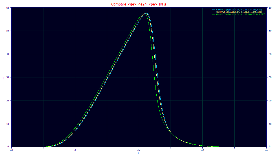
The above plot shows a GenHVL with a <ge> IRF in blue, and <e2> IRF in yellow, and a <pe> IRF in green. In each case the wider exponential was constant and the narrow component was adjusted to give the same attenuation. The trend from the <ge> to the <e2> to the <pe> is clear. The differences are subtle, and do not impact the actual far-tailing (which is governed by the higher width exponential). To effectively fit these different IRFs and see a difference in this narrow width component, you will need a high sampling rate and the peaks should have as high as S/N as possible without entering into an overload state. Also a high a3 chromatographic distortion will produce an intrinsic fronting or tailing which will more cleanly render the IRF isolatable (non-correlated) in the fitting.
Single-Component IRFs
Although we explored over a hundred different IRF models for PeakLab, we largely ceased using single-component IRFs except for data which had a poor S/N where the data could support fitting only the higher-width component. In such instances, the exponential <e> IRF was almost always the most appropriate. Although PeakLab includes a number of single component IRFs, these should be deemed experimental.
The <e> IRF
Since the two-component IRFs strongly fit the fixed delay with this first order exponential, using the <e> single-component first order exponential IRF will generally result in this system or variable component of the IRF either not being fitted, or possibly being somewhat accounted by the primary a3 chromatographic distortion and/or the a4 asymmetry in the GenNLC and GenHVL models, rendering these model parameters much less accurate.
Omitting the IRF in Peak Fitting
Fitting an isocratic peak to a closed-form model (without an IRF) which has not seen the removal of the IRF in a preprocessing step is not recommended. The fit is likely to be poor, all of the parameter estimates will be less accurate.
If you are addressing overlapping and hidden peaks, even if you are only seeking to recover the areas of specific components, an IRF preprocessing step is usually beneficial. While it may not be possible to fit a model with an <irf> if there is not a clean delineation of the tailing, if the system's (instrument/column/prep) IRF is known, a Fourier deconvolution of the IRF may make the overlapping or hidden components appreciably clearer and easier to fit.
Gradient HPLC
In the instance of gradient HPLC, the IRF and gradient are usually inseparable if the peak elutes during the gradient. A gradient peak's IRF will mostly vanish in the gradient, giving the appearance that no IRF exists. It does exist, but the IRF tailing will be offset and hidden and statistically inaccessible in <irf> bearing fits. Even if a twice-generalized model (one accounting both the skew or third moment, and kurtosis or fourth moment) makes it possible to recover the theoretical diffusion or kinetic widths, and the chromatographic distortions, those values will be impacted by both the gradient and the masked IRF in direct fits of the gradient shapes.
Is IRF Determination Difficult?
In certain cases, it is so simple as to be nearly effortless. Since an IRF representing instrumental non-idealities introduces delays and thus additional tailing in a peak, fitting a standard which includes a peak that elutes with any measure of intrinsic fronting (the chromatographic distortion will be in the opposite direction), however small, is often sufficient to accurately quantify the IRF, especially when the S/N is good and the baseline subtraction is accurately made. In the worst case scenario, you may need to add an early eluting component to your standard in order to have an intrinsically fronted peak for IRF estimation. In IC cation studies, we found a consistent threshold of retention where all earlier eluting peaks were intrinsically fronted.
Approaches for IRF Determination
We describe the IRF Estimation process in detail in a sequence of decreasing preference. It is very possible you will not need anything more than this first approach.
IRF Estimation 1 - Standards Containing One or More 'Fronted' Peaks
IRF Estimation 2 - Standards Sectioned to Contain Only Fronted Peaks
IRF Estimation 3 - Standards Containing Only Tailed Peaks
We also describe considerations of specific interest to GC: