
PeakLab v1 Documentation Contents AIST Software Home AIST Software Support
3D DAD Chromatography
DAD Import Data Format
To input the specific chromatographic or spectral data from a DAD matrix of data, the following structure is required:

The data must be a matrix stored as an ASCII CSV file (use Excel's default CSV export if necessary) with the first cell empty, the wavelength values in the first row, the time values in the first column, and the DAD information in the matrix between.
Import Chromatography from DAD 3D Data Matrix
This option is useful for extracting the chromatography for specific wavelengths of interest. These can be imported from multiple 3D matrices and multiple WLs, up to 24 data sets in a single step. When the File menu's Import Data Sets(s) | DAD 3D Chromatography | Import Chromatography from DAD 3D Data Matrix... option is selected, the following dialog appears:
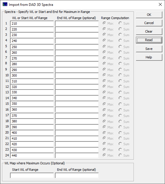
The simplest import is shown above. Only the first WL column is used. In this example, the spectra from 210 to 440 are extracted from the matrix, and 24 data sets are generated. In this example, the import configuration was applied to a single 3D matrix. This may be useful for a more thorough exploration of the spectral-time surface.
The following plots use the 3D functionality in the View and Compare Data option to furnish strong 3D visualizations of the 24 chromatographic extracts from the time - WL spectra. The 3D gradient (ribbon), shaded, and contour plot visualizations are shown below:
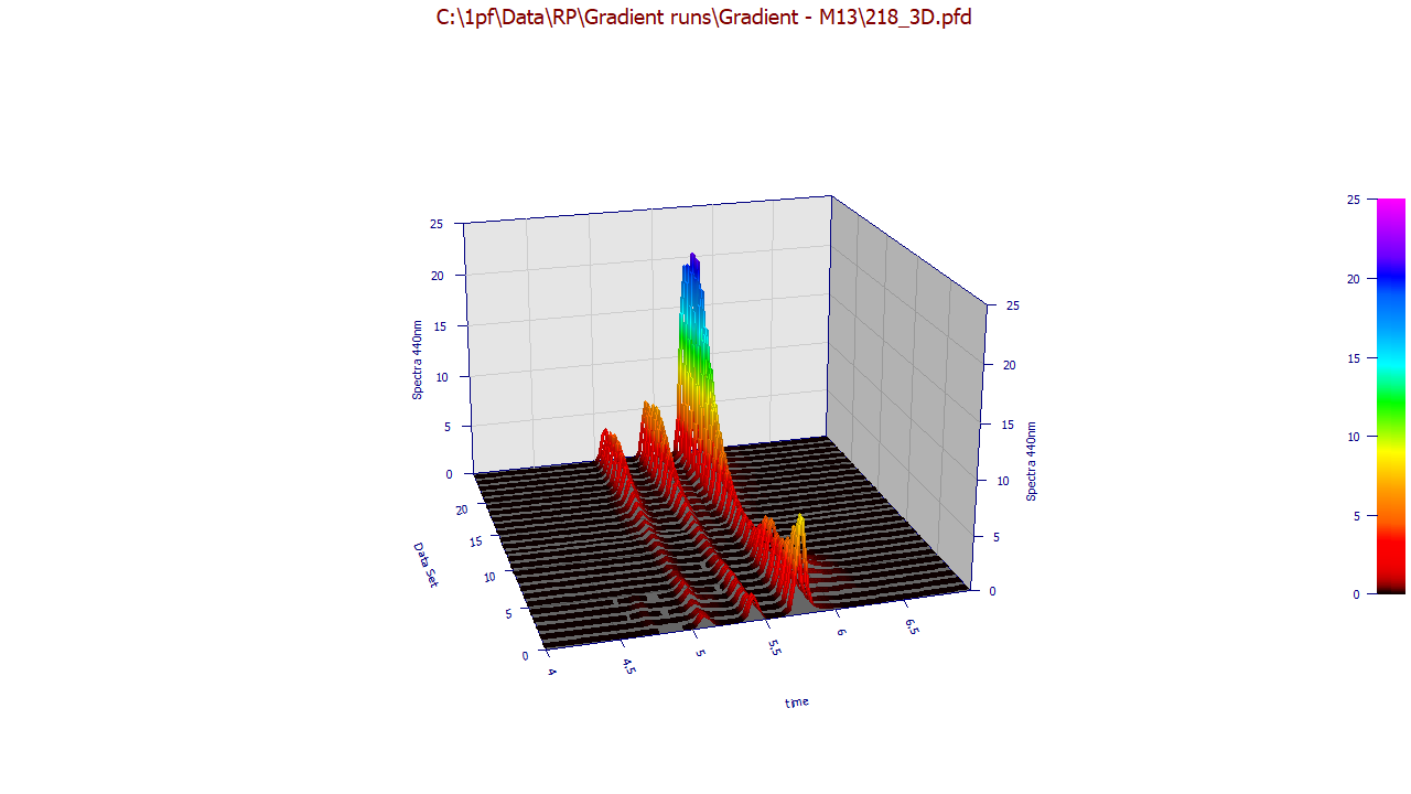
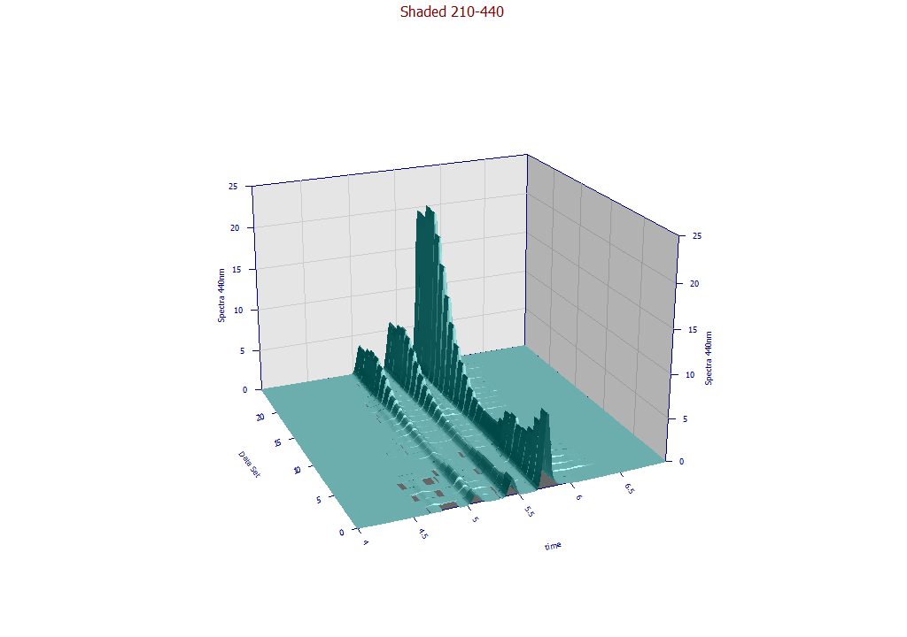
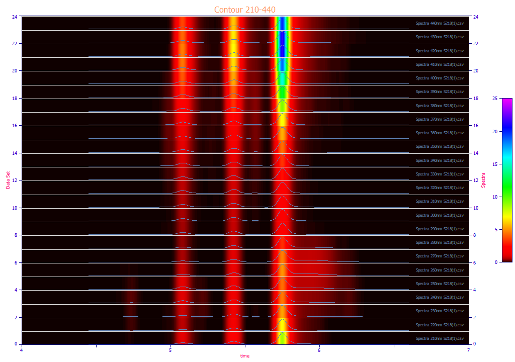
The contour patch plot option also plots a normalized chromatographic trace at each of the wavelengths in the plot. To zoom in a portion of the surface, it is often easiest to do this on the contour plot and then change to the 3D surface plots.
Extracting Maximums and Integrated Values in Wavelength Bands
If a range is specified with a starting and ending WL, you must select either the maximum (Max) or the sum of the spectral values (Sum) from the beginning to the ending WL specified. If you specify a WL range from 210 to 240, and Max as the operation, the resultant spectra will be the maximum DAD spectral value across this WL band for each point in time. Each spectral value may correspond with a different WL, the one where the maximum occurs at that point in time.
If Sum is selected, the spectra will consist of an integration from the starting to ending WL.
WL Map where Maximum Occurs
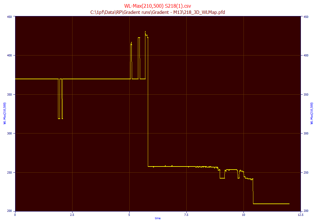
It can be useful to see the WL where the maximum occurs at each peak that is seen between any range of wavelengths. In this example, we specify 210 for the start and 500 for the end WL. This map will contain the WL value where the maximum occurs at each point in time in the elution. This can be a convenient way to isolate and identify components:
Digital Filtering
In this example, an Agilent DAD matrix with a 1 nm wavelength increment was used. When a 240nm wavelength is specified, the exact 240nm chromatography is extracted from the data matrix. Note that this may not exactly match the 240nm chromatography specified in the separation. In the case of the Agilent instruments, there will be a Gaussian convolution DSP denoising filter that is applied to the WL-specific chromatography. In our experience, the S/N will be slightly higher on the WL-specific data used in the instrumental analysis. This digital filter will also add a slight measure of Gaussian character that was not present in the actual separation, and this will to a small measure impact each of the fitted parameters in a generalized chromatographic model. Again, it is our experience that the digital filtering alters the fitted parameters; you will not see an exact match between the DAD extract and the specific WL data from an instrumental analysis. We will also note that the higher S/N and the denoising distortion tend to offset one another; the goodness of fit of a very well-fitted peak does not improve when using the DSP filtered data.
Interpolation
There may be instances where you need an interpolated WL value. An example would be where the first derivative technique is used to quantify coelutions and the DAD matrix consists of Savitzky-Golay first derivative (by WL) spectral values. Please see the Fitting Coeluting Peaks tutorial for more information. If a WL such as 240.275 is specified, for example, a bivariate spline surface (bicubic) is used to generate an interpolant that will be used to produce an interpolated WL spectra. Note that the Range Computations are not available when interpolation is being used. Those columns will be grayed out and inaccessible when the specified WL is not one of those within the actual matrix. Also, only interpolation is available. The available wavelengths are limited by the bounds of the matrix.
Import Spectroscopy from DAD 3D Data Matrix
This is especially important for separations where the overlap in the fitted peaks in a chromatographic data set is incomplete and you can determine, from the fitting, that a single component exists between a given t1 and t2. This option allows you to extract the UV-VIS spectra for the pure component that was eluted during that time interval. When the File menu's Import Data Sets(s) | DAD 3D Chromatography | Import Spectroscopy from DAD 3D Data Matrix... option is selected, the following dialog appears:
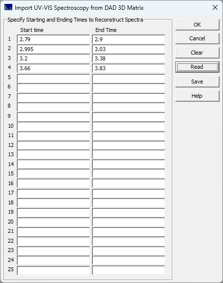
In this example, four distinct but chemically similar compounds are specified by their chromatographically exclusive time intervals in the separation:
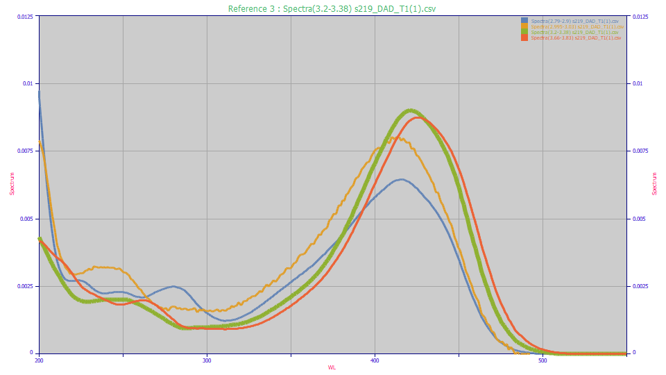
These UV spectra can then be fitted in PeakLab using Gaussian or Voigt functions in the Spectroscopy family. For comparison purposes, here we use the Unit Area option in the View and Compare Data option to see the four distinct UV and VIS principal absorptions. Note that low concentration peaks near the baseline (such as the amber curve) will have noisier spectra and those may require the Smooth option to get a clear picture of the peak wavelengths.
If you are using the first derivative method to remove one component of two coeluting peaks, you can use this approach with pure standards to get the UV-VIS maxima and minima wavelengths of each without running a separate analysis with a dedicated UV-VIS spectrometer. By using the chromatographic instrument's DAD to determine the exact wavelengths, these should be precisely the wavelengths needed in chromatographic analysis.
View/Reduce DAD Data Matrix
If you wish to visualize portions of the DAD matrix or reduce its size using only a portion of the overall UV-VIS wavelength bands, or reduce the time sampling if there are too many time samples, you can use the File menu's Import Data Sets(s) | DAD 3D Chromatography | View/Reduce DAD Data Matrix... option. After selecting the CSV ASCII DAD data file, you will see the following dialog:
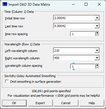
Pay close attention to the size of the grid. PeakLab does not reduce the grid for fast surface rendering. The intention is to visualize everything in the data you are exploring. You will probably find the visualization most palatable if you can keep the size of the grid to less than 100,000 points. By default, the Agilent UV-VIS ASCII export will have 611 signal values at each time (from 190nm to 800nm at 1 nm intervals). For this data set with 1200 time values across 6 minutes, that is close to 550,000 points, as shown above. If you were able to sample at a high enough sampling rate with the 3D option enabled, you may be able to change the time row spacing to every other point (2), or select a start and end time for just the eluted components of interest. In many cases, the wavelength band can be limited to just the UV.
If you wish to have this filtered matrix available for future work, you can use the Export option to save the surface as either a reduced size ASCII matrix, or an ASCII XYZ file (where each entry is a point in the grid).
When you click OK, there will be a short delay as the surface is prepared. Unless you check Omit smoothing in surface generation, the matrix will be smoothed in the time dimension using a default Savitzky-Golay denoising filter at each wavelength in the matrix. The surface is then rendered with the Renka C1 surface interpolant. Unless the times and wavelengths have been substantially narrowed, the initial unzoomed plot may contains hundreds of patches (if a patch plot is being rendered). In general, you will need to zoom in the plot to see the time and wavelength regions of interest.
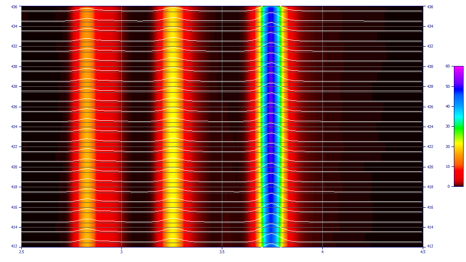
Options of interest may be:
![]() The Modify Contour Properties button in the graph toolbar opens the option to turn the patch plot
option on and off and to set the resolution of the contour plot.
The Modify Contour Properties button in the graph toolbar opens the option to turn the patch plot
option on and off and to set the resolution of the contour plot.
![]() The Overlay Data on Surface or Contour button in the graph toolbar displays and hides the normalized
traces of the chromatography.
The Overlay Data on Surface or Contour button in the graph toolbar displays and hides the normalized
traces of the chromatography.
![]() The 2D View options can be used to set a stronger line width and antialias to better see the traces.
The 2D View options can be used to set a stronger line width and antialias to better see the traces.
![]()
![]() You can use the 3D gradient and shaded options with the
You can use the 3D gradient and shaded options with the ![]() 3D animation to better visualize the surfaces.
3D animation to better visualize the surfaces.
![]() You can use the Render 3D Surfaces with Plateau at Upper Z Bound to close the surface at the rendering
bound
You can use the Render 3D Surfaces with Plateau at Upper Z Bound to close the surface at the rendering
bound
![]() The Logarithmic Z Axis will possibly highlight trace components in the baseline at certain wavelengths
and times:
The Logarithmic Z Axis will possibly highlight trace components in the baseline at certain wavelengths
and times:
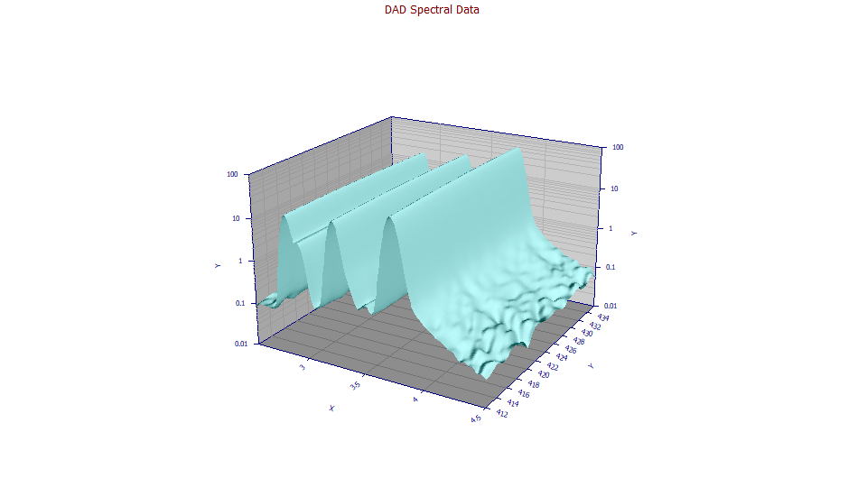
The Force | Zmin = 0 will set the lower limit of the plot at a fixed 0.0, ignoring negative values. This is also useful for seeing peaks in the baseline.
The Force | Zrange = -1,1 will set the lower limit of the plot at a fixed -1 and the upper limit of the plot at +1. This will typically amplify baseline detail.
Extrema
The initial values in the Extrema section will represent the incoming data matrix values. When the plot is zoomed, and the Update button is clicked, the minima and maxima will be updated for the for the zoomed surface with the narrower bounds and the higher resolution. The extrema are based on the values taken from a 250,000 point grid based upon the zoomed x and y ranges. The actual values of these extrema will depend (1) on the optimal Savitzky-Golay filter applied to the incoming DAD data (if used), (2) on the 250,000 point (500 x 500) evaluated Renka C1 3D interpolated surface (this resolution is independent of the grid used for the rendering of the contour or 3D surface plot), and (3) on the level of zoom which determines the x and y bounds of that 250,000 point grid.
Partial Derivative Surfaces
The Renka 3D rendering algorithm offers a C1 partial derivative surface with respect to either time (dZ/dX) or wavelength (dZ/dY). These are useful for visualization, and can often have a good accuracy in estimating the wavelengths where the first derivative with respect to wavelength are zero.
Export
This option will export the data matrix used for the extrema computations. It will always consist of 500 equally spaced wavelengths, and 500 equally spaced time values, within the zoomed in region that is plotted. The initial values in the Extrema section will represent the incoming data matrix values. You can save a matrix or a table of XYZ values. Although you can use this option to export a first partial with respect to wavelength surface for derivative fitting, we recommend the next procedure for best accuracy in estimating coeluting peak areas.
Create First Derivative DAD Matrix
Please see the Fitting Coeluting Peaks tutorial for a using identified zero first derivative wavelength values for estimating the areas of coeluting peaks with slightly different UV-VIS spectra. The File menu's Import Data Sets(s) | DAD 3D Chromatography | Create First Derivative DAD Matrix... option will use a default Savitzky-Golay filter optimized for first derivatives. The matrix is generated with the same time and wavelength values as the incoming data. There is then an option to directly plot the partial derivative surface.
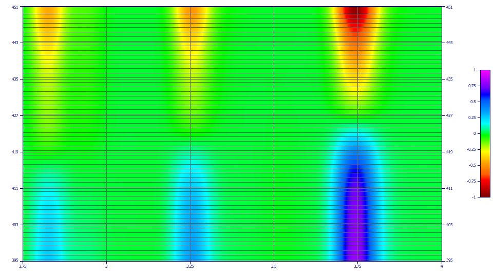
This option has been designed to produce accurate first derivative spectra. The Savitzky-Golay smoothing is necessary to produce the derivative matrix and cannot be disabled. To confirm the wavelengths where a given component will be zeroed, zoom in the zero band on each component where you want to identify the wavelength and click Update. The Min(Abs(Z)) Y value will be the pertinent D1=0 wavelength value. The zero zone is easy to locate in a patch plot since the D1 peak is inverted on one side of the zero point. The D1 location is also the mode or apex location in the non-derivative data. It may be easier to get this value directly from a reference standard where just one of the two coeluting components is present. It may also be possible to get the spectra of the individual components from time regions in a high-resolution chromatographic separation where the two components have no overlap with one another.
Create Composite Matrix from Multiple DAD Data
If you have saved all replicates as 3D data, you can use the File menu's Import Data Sets(s) | DAD 3D Chromatography | Create Composite Matrix from Multiple DAD Data... option to create a composite single matrix containing the sum of the spectral values for each of the replicates. Since the raw DAD instrumental data can have the same sampling rate, but other than a pure 0 starting time value, this option only requires that the count of time and wavelength values match across the different matrices. The actual times will come from the reference matrix shown in the conversion status dialog. You will see a warning when the starting time values are not constant across the replicates. This procedure also presents a viewing option after the composite matrix is generated.
A Special Thank You
AIST Software would like to personally thank Dr. M. Farooq Wahab at the University of Texas at Arlington for his motivation to use improvised techniques as it appears in PeakLab. Dr. Wahab echoed our sentiments that novel 3D diode array detector analyses are seriously underused in science. It is our hope that by making this first derivative coelution analysis as close to effortless as possible, its use will become more widespread in the chromatographic sciences. Dr. Wahab furnished us with a 1995 report from the Analyst, Real-time Analysis of Multicomponent Chromatograms: Application to High-performance Liquid Chromatography, which we believe is the first report of this method.
 |