PeakLab v1 Documentation Contents AIST Software Home AIST Software Support
White Paper: Part III - HPLC Gradient Peaks
Part III - HPLC Gradient Peaks
In Part I of this series we described a generalization of the HVL and NLC models which accommodated higher moment differences in the zero distortion (infinite dilution) density underlying the peak shapes in chromatographic separations. In Part II, we added the complexity of fitting the mathematical convolution of this 'true' peak model and an IRF, or instrument response function, in the fitting of analytical isocratic peaks. In Part III, we will now address the further complication in the shape of chromatographic peaks when the strength of the mobile phase is changing in gradient HPLC separations.
Gradient HPLC - Convolution and Deconvolution
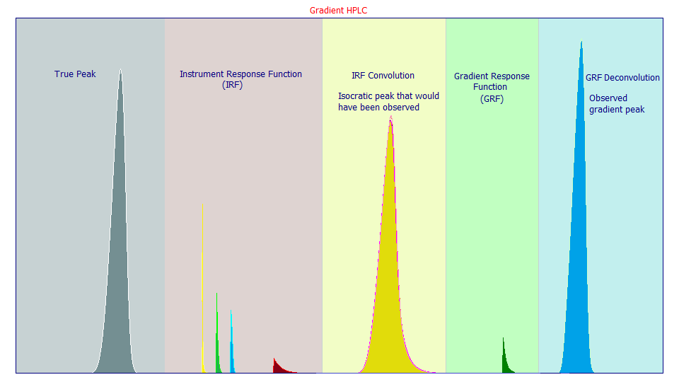
To the already complex process of chromatographic modeling, gradient separations require that we add a deconvolution step after an isocratic peak is generated as we described in Part II of this white paper series. In this additional step, the isocratic peak that would be observed by the instrument is replaced by a deconvolution which cancels a measure of the right-side tailing distortion introduced by the IRF. In this case, the HPLC gradient cancels out much of the influence of the IRF, while also dramatically compacting the tails of the observed peak. We have found an HPLC gradient to be well-modeled by a half-Gaussian deconvolution, as shown in the graphic below. Given that much of the isocratic IRF tailing arises from the higher width first order kinetic (the red IRF component below), a half-Gaussian deconvolution will not produce a true cancellation, merely an additional alteration, a further complication, to the observed peak arising from this deconvolution describing the gradient compression of the peak shape.

Gradient Peak Shapes
In gradient HPLC, the once-generalized chromatographic peak models used for isocratic elutions will not work, with or without an IRF in the model. The changing strength of the gradient across the time of elution for a peak will fundamentally change its shape, producing a more compact tailing. In order to effectively fit gradient HPLC peaks, this more compact fourth moment tailing must be accounted in some manner.
This fourth moment tail compression can be addressed in at least three different approaches:
1. You can ignore both the instrument response function (IRF) and the gradient response function (GRF) and directly fit the gradient peak shape using a twice-generalized chromatographic model capable of managing the compressed tails as seen in the observed peak (the blue shape above). This will allow an estimate of the strength of the gradient via the parameter consisting of the power of the tail compression, or the via the measured fourth moment, but this direct twice-generalized model fit will not theoretically estimate the GRF, the response function for the gradient.
2. You can ignore the IRF and fit a GRF deconvolution model instead of an IRF convolution model. In a deconvolution model, the blue observed gradient peak is separated into a gradient response function (the green GRF above) and an implied isocratic shape. Since a portion of the right asymmetry in the IRF is destroyed by the gradient, this implicit isocratic peak will not be the yellow peak shown above (where the full IRF is shown), but rather a peak with only a remnant IRF, one containing only that portion of the IRF which survived the gradient. Because much of the IRF that would be present in an isocratic separation is not present in this implicit isocratic shape estimated in the deconvolution fit, and since the deconvolution unwinds the fourth moment tail compression to a natural power of decay, a once-generalized model can successfully describe this implicit isocratic shape arising in the deconvolution.
3. Once a GRF for a given procedure has been estimated, you will have a parametric description, a deconvolution model, for the gradient. This can then be used to unwind the gradient in a Fourier convolution preprocessing step for any data set that employs this same gradient. The blue and green curves are convolved in the Fourier domain directly to produce the implicit shape described in the deconvolution modelling of approach 2. In this case, an unwound peak is not a implied object in a one-step deconvolution fit, but it is the actual output observed from a Fourier convolution. Each unwound peak will be the true isocratic peak and the non-cancelled portion of the IRF. This shape can then be fitted to a once-generalized model with or without an IRF. We know that a small portion of the wide component of the original IRF (the red distortion above) will survive the gradient. We again note that working in reverse from the blue gradient peak, convolving the green GRF, will unwind the tail compression but it will not restore the yellow isocratic peak shown above that would have been observed in a non-gradient separation. An unwound gradient peak will contain only the uncanceled portion of the opposing convolution and deconvolution response functions. In most instances, this remnant IRF can be ignored and a very fast closed form once-generalized chromatographic model fitted. If a significant measure of the wide exponential of the original IRF is not sufficiently cancelled by the gradient, you may be able to fit the unwound gradient data to a model bearing a one-component <e> IRF, a single exponential.
Approach 1: Direct Closed Form Fits of the Gradient Peaks which Fit the Tail Compression as a Fourth Moment Effect
The simplest approach to modeling gradient peaks is to use a twice-generalized model such as the Gen2HVL which adjusts both the third and fourth moments of the ZDD zero distortion density. It is one of the easiest of all possible peak fits once the data have been extracted from the sloping gradient baseline. This approach requires nothing more than choosing a twice-generalized model to fit the peaks.
In Part I, we covered the once generalized HVL where a third-moment or skewness was added to the zero distortion density (ZDD) used in the model. We illustrated the GenHVL model where a generalized normal furnishes this third moment asymmetry in the infinite dilution density, and we also covered the fact that this model also manages the Wade-Thomas NLC kinetic model chromatographic shapes.
For a twice generalized model that also adjusts the fourth moment or kurtosis, the 'fatness' of the tails, a more involved ZDD model is needed. We derived the generalized error model for this purpose. It is essentially a generalized normal, with an error model power of decay:
a0 = Area
a1 = Center (as mean of asymmetric peak)
a2 = Width (SD of underlying Gaussian)
a3 = Power of Decay of Tails, controls kurtosis or fourth moment
a4 = Asymmetry ( fronted -1 > a3 > 1 tailed), controls skew or third moment
By inserting this Generalized Error Model ZDD for the PDF, CDF, and CDFc in GenHVL template, we produce the Gen2HVL model:
a0 = Area
a1 = Center (as mean of the ZDD)
a2 = Width (SD of underlying normal ZDD)
a3 = HVL Chromatographic distortion ( -1 > a3 > 1 )
a4 = Power n in exp(-zn) decay ( .25 > a4 > 4 ) adjusts kurtosis (fourth moment)
a5 = ZDD asymmetry ( -1 > a5 > 1 ), adjusts skew (third moment)
Note that the a5 value controlling the skewness of the ZDD in the Gen2HVL peak appears as a4 in the ZDD nomenclature, and the a4 value controlling the power of the decay of the tails in the ZDD of the Gen2HVL peak appears as a3 in the ZDD nomenclature. For consistency in a chromatographic model, a3 is always the concentration-dependent chromatographic distortion of the HVL and Wade-Thomas NLC models.
In this type of modeling, the gradient shape is fitted directly. There is no effort to specifically model the gradient. The mix of IRF and gradient effects, whatever remains, is fit with the higher order moment adjustments in these twice-generalized models.
This works because any IRF that would be present in isocratic elutions (or in an isocratic hold in a gradient run), is mostly lost in the compression of the gradient. A closed form model is fit because it is not usually possible to fit an <irf> bearing model directly to gradient peak shapes. Here one is directly fitting a distorted shape using the higher order parameters in a Gen2HVL or Gen2NLC model to address the gradient-introduced asymmetry, the gradient-introduced compression, the various remnants of the IRF, and the deviations from the theoretical zero distortion density idealities.
In gradient peaks, the instrumental IRF and the gradient GRF are in opposite directions. The IRF adds tailing, the gradient removes it. The net effect is a shape that can be somewhat successfully fitted with a two higher-moment (third and fourth) generalized chromatographic model.
In fitting a Gen2HVL or Gen2NLC directly to baseline corrected gradient data, the third moment a5 parameter will probably be addressing the gradient effect far more than any multiple site deviation from the theoretical expectation of an infinite dilution density. Insofar as the kurtosis or fourth moment is generally close to constant in isocratic elutions, the a4 fourth moment parameter in a gradient peak fit will almost exclusively map the change in strength of gradient across the time of the peak's elution.
In this simplest strategy for gradient fitting, it is all about a model whose parameters map as much of the orthogonality (independence, lack of correlation) of moments as possible.
Gaussian
Because a well-designed gradient separation will produce close to symmetric peaks, there is sometimes the assumption such peaks are indistinguishable from Gaussians.
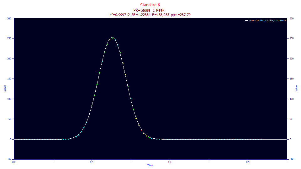
While it is true that the Gaussian model will generally fit gradient peaks much better than isocratic ones with an unattenuated IRF, the fits will be far from optimal. In the Gaussian fit to the gradient peak standard above, the error is 288 ppm. Although it is not apparent without the fit as a reference, there is a slight asymmetry that is not accommodated. The tails are also compressed from the gradient, something very difficult to see visually.
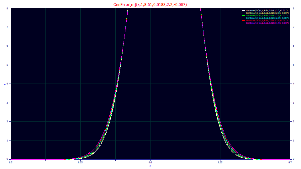
The above plot consists of the generalized error ZDD with the power of decay varying from 1.95 to 2.20. This ranges from a typical lower bound for an isocratic peak to a typical upper bound for gradient peaks. The difference in the kurtosis or fourth moment is mostly in the tails. A peak can appear Gaussian to the eye, but it isn't easy to visualize the thickness of the tails and errors which occur near the baseline of peaks.
Gen2HVL
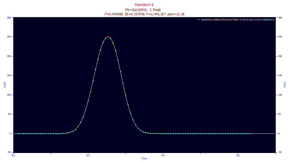
This is the Gen2HVL fit to this same gradient peak. By adding the a3 chromatographic distortion, an a4 tailing power in the ZDD, and an a5 asymmetry in the ZDD, the fit now has an error of 12.2 ppm and the F-statistic which is often use a statistical gauge of the efficacy of the modeling, requiring each additional parameter to make a significant contribution, increases from 184,600 to 1.13 million, about a six-fold improvement.
Fitted Parameters
r2 Coef Det DF Adj r2 Fit Std Err F-value ppm uVar
0.99998782 0.99998698 0.25704830 1,445,267 12.1775257
Peak Type a0 a1 a2 a3 a4 a5
1 Gen2HVL 11.0095917 8.32532591 0.01749026 -5.734e-06 2.11375432 -0.0046614
Measured Values
Peak Type Amplitude Center FWHM Asym50 FW Base Asym10
1 Gen2HVL 249.661481 8.32690109 0.04187012 0.93998477 0.08103660 0.94393202
Peak Type Area % Area Mean StdDev Skewness Kurtosis
1 Gen2HVL 11.0095917 100.000000 8.32608408 0.01714848 -0.0374068 2.89627570
Parameter Statistics
Peak 1 Gen2HVL
Parameter Value Std Error t-value 90% Conf Lo 90% Conf Hi
Area 11.0095917 0.00471211 2336.44552 11.0017585 11.0174249
Center 8.32532591 0.00012725 65423.1018 8.32511437 8.32553745
Width 0.01749026 8.3495e-06 2094.77338 0.01747638 0.01750414
Distortn -5.734e-06 1.0184e-06 -5.6303887 -7.427e-06 -4.041e-06
Q-power 2.11375432 0.00321213 658.054080 2.10841463 2.11909402
Z-Asym -0.0046614 0.00258036 -1.8064978 -0.0089509 -0.0003719
What do these three additional parameters beyond a Gaussian contribute to one's understanding of the chromatography? The a3 chromatographic distortion, is of a very low value, as fitting the ultra HPLC concentrations. It is of a negative sign, which suggests the peak is intrinsically fronted with respect to concentration dependency. The peak's ZDD or zero distortion density is almost symmetric, a very slight left skewed -.0047 a5 statistical asymmetry. We believe the a5 term has far more to do with the state of the gradient than the third moment ZDD considerations in isocratic peaks. If we fit the once-generalized GenHVL which lacks this additional fourth moment adjustment, the goodness of fit is 150 ppm, and the F-statistic actually decreases from the 158,000 of the Gaussian to 147,851. This is important; it means that adding the chromatographic distortion and a ZDD asymmetry adjustment did not improve the efficacy of the fitting. This fourth moment adjustment is essential for a close-to-zero error direct fit of a gradient peak shape.
If you look at a4 above, you see a value of 2.11. If you look at the estimated fourth moment, the kurtosis, you see 2.896. A pure Gaussian decays at a power of 2.0, and with a kurtosis or fourth order 'fatness of tails' of 3.0. The higher than 2.0 power of decay and the kurtosis below 3.0 means the peak's tailing is compacted by the gradient. So long as a set of gradient peaks have close to the same width, as is often true in well-designed gradient separations, the a4 parameter value, or possibly the actual fourth moment kurtosis, can be used as an estimate of gradient strength.
In this type of fitting, each peak's compression is estimated. There is thus an estimate of gradient strength at each point in time where a peak is estimated. If a gradient varies across time, this will be reflected in these estimates. This approach is as effortless as fitting simple Gaussians, and with a closed-form model, even if it appears far from simple as in the case of the Gen2HVL shown above, the fits are generally close to immediate. For example, a 1000 point data set containing eleven gradient peaks fits to 11 Gaussians in .34 sec, and to 11 Gen2HVL peaks in 1.82 sec. Once or twice-generalized models, closed form, no IRF, fit quite swiftly.
Approach 2: Estimating the Gradient by Fitting a Deconvolution
With this step we introduce a new software technology, 'deconvolution' model fitting, that can be used for discovering the gradient's system response model and parameters.
The basic IRF-bearing GenHVL<g> model, for example, fits a convolution of the GenHVL model with the <g> half-Gaussian response function to data. The data is assumed to be smeared and distorted by the half-Gaussian instrument response function. The parameters of the fit recover the pure model absent the IRF.
The GenHVL<*g*> model, on the other hand, does just the opposite. It fits a deconvolution of the GenHVL with the <g> half-Gaussian response function, estimating the <g> system parameter for the gradient. The gradient data is treated as deconvolved (sharpened) data as opposed to convolved (IRF-smeared) data. In this instance, the parameters of the fit recover the estimates describing the gradient as well as the estimated peak parameters with the gradient removed.
In this 'reverse' type of fitting, there is the issue of noise. The very low sample gradient HPLC concentrations produce peaks with a measure of noise, and a deconvolution only adds further noise, even with a Fourier-domain filter automatically applied.
Deconvolution models are 'gradient discovery' models which are generally used with single peak gradient standards for the purpose of identifying the gradient's system response function and deriving estimates for its parameters. Interestingly, since peaks are placed based on the raw data, and the gradient peaks have a sharpened state, the loss of resolution from a 'unwinding' convolution and subsequent fitting, as occurs in approach 3, is not a factor in this form of fitting.
The only system response models we have found to accurately describe an HPLC gradient were the <*g*> (with a retention unit SD width of approximately .015-.02) and the variable order kinetic <*k*> (with an order of 0.6-0.7 and a time constant width of 0.015-0.02 retention units).
Fitted Parameters
r2 Coef Det DF Adj r2 Fit Std Err F-value ppm uVar
0.99999913 0.99999907 0.06869090 20,238,780 0.86961687
Peak Type a0 a1 a2 a3 a4 a5
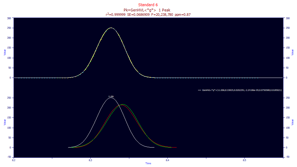
1 GenHVL<*g*> 11.0059759 8.33825080 0.02022911 -2.242e-5 0.07505876 0.01850210
A deconvolution fit can be quite effective. Fitting the GenHVL<*g*> results in an estimate of the gradient as a half-Gaussian response of 0.0185 and with a fit having less than 1 ppm unaccounted variance error.
You will note that a deconvolution fit is the reverse of an isocratic fit with an IRF. The white peak above is the gradient shape, the red peak is the unwound peak absent the influence of the gradient, and the green is the estimated pure HVL peak had an isocratic separation occurred. Note that even with a very low a3 chromatographic distortion, there is still a difference between the unwound GenHVL peak in red and unwound HVL in green.
In using this fitting method to estimate the gradient's system response function, you will probably need to set initial parameter values that do not produce negative values in the deconvolutions shown which attempt to match the raw data peaks. While in fitting it is often advantageous to set starting estimates higher than the expected fit values, this is an exception since it can produce local minima fitting issues.
Approach 3: Unwinding the Gradient and Fitting a Once-Generalized Model
If the gradient is perceived as a non-linear transform that compresses a peak, one can use Fourier convolution to unwind or undo the gradient, approximating the peak that would exist if the gradient had not occurred. Unlike the IRF deconvolution, where one seeks to remove a distortion to recover the true peak, here we seek to recover the true peak by adding back that which occurred within the gradient. In other words, we treat the gradient process as a deconvolution which narrows the peak, and we apply a convolution to restore the original width and shape of the peak. We treat the gradient process as a deconvolution which is undone by a subsequent convolution with an IRF which represents its system response function.
In the spirit of allowing the data to reveal the nature of the system IRF altering it, we can take the simple approach of convolving different IRFs to see if a peak shape can be restored which can be more accurately fitted with an isocratic model. We can make the inference that the better an isocratic model is fitted, the closer we are to the response function that represents the gradient process.
If the gradient process is a purely linear one, we can use a zero order kinetic model to restore the peak shape. If the gradient process is first order, we can use an order 1 kinetic model. We can convolve any order kinetic model we wish. We can also fit a probabilisitic IRF. If we assume the gradient process is a one-sided Gaussian deconvolution, we can restore the original peak shape by convolving a simple half-Gaussian response function.
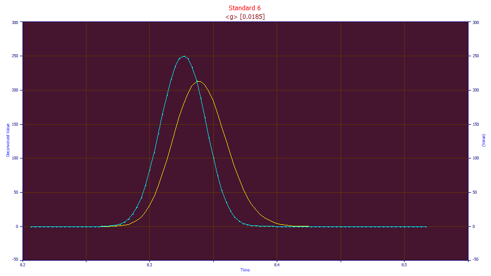
In this example, we apply a simple one-parameter Gaussian convolution data to the data set (in blue above). If this fit of the convolved data (the yellow curve) is significantly improved, we can assume we have unwound at least a portion of the gradient without introducing more harm than benefit. In fairness, convolution does smooth data, so we will see a modest improvement from this noise reduction, but only so long as the new shape is at least as applicable as the original to the model used in the fitting.
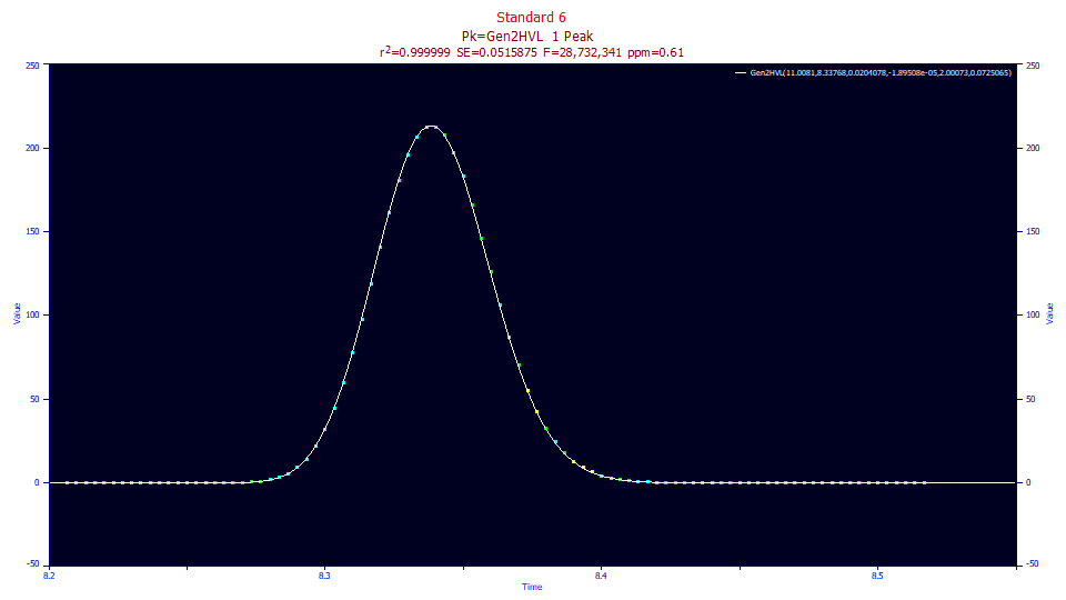
The half-Gaussian convolved data fits to an even better goodness of fit than the deconvolution model, 0.61 ppm unaccounted variance.
Fitted Parameters
r2 Coef Det DF Adj r2 Fit Std Err F-value ppm uVar
0.99999939 0.99999935 0.05158750 28,732,341 0.61254977
Peak Type a0 a1 a2 a3 a4 a5
1 Gen2HVL 11.0081240 8.33767593 0.02040778 -1.895e-05 2.00073302 0.07250650
Parameter Statistics
Peak 1 Gen2HVL
Parameter Value Std Error t-value 95% Conf Lo 95% Conf Hi
Area 11.0081240 0.00104448 10539.3082 11.0060483 11.0101997
Center 8.33767593 5.8828e-05 1.4173e+05 8.33755902 8.33779284
Width 0.02040778 8.064e-06 2530.73013 0.02039175 0.02042380
Distortn -1.895e-05 5.1353e-07 -36.903388 -1.997e-05 -1.793e-05
Q-power 2.00073302 0.00075144 2662.53272 1.99923969 2.00222635
Z-Asym 0.07250650 0.00075486 96.0533212 0.07100638 0.07400662
In this instance, we fit a twice-generalized Gen2HVL to confirm the successful unwinding of the gradient with this 0.0185 estimate of the half-Gaussian deconvolution gradient response function. Here we see close to a perfect 2.0 power of decay in the a4 parameter.
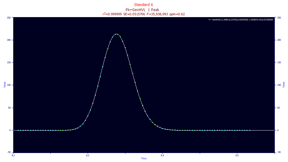
If we fit the once-generalized GenHVL, where this 2.0 power of decay is built-into the model, we realize nearly the same 0.61 error, but the F-statistic is now 35 million. We can contrast this with the 1.4 million of the direct twice-generalized Gen2HVL fit to the gradient shape. With this overall accuracy of sub 1-ppm error, we can assume the parametric estimates of the primary a0-a3 chromatographic parameters are highly accurate.
Fitted Parameters
r2 Coef Det DF Adj r2 Fit Std Err F-value ppm uVar
0.99999938 0.99999935 0.05157059 35,938,993 0.61910433
Peak Type a0 a1 a2 a3 a4
1 GenHVL 11.0084338 8.33764652 0.02040377 -1.921e-05 0.07285693
Equivalent Parameters
Peak Type a0 a1 a2 a3 a4
1 GenNLC 11.0084338 8.33764652 2.4966e-05 -1.921e-05 29.7717160
Measured Values
Peak Type Amplitude Center FWHM Asym50 FW Base Asym10
1 GenHVL 213.298719 8.33854147 0.04850680 1.03756466 0.09693624 1.09954591
Peak Type Area % Area Mean StdDev Skewness Kurtosis
1 GenHVL 11.0084338 100.000000 8.33987414 0.02062568 0.16454728 3.05044827
If the unwound fit values are compared to those of the deconvolution model, all of the parameters are very close to identical, including the a4 asymmetry.
Although the a4 ZDD asymmetry is quite high and positive, and the third moment skewness is a right-sided 0.164, the a3 chromatographic distortion is negative, an intrinsically fronted peak. Note that this fronted character (negative a3) was observed with the examples we made with all three approaches, including the direct fit of the gradient shape.
The 0.073 a4 ZDD statistical asymmetry is a higher value (0.015 is more typical for an isocratic peak), and likely reflects the fitting of the IRF surviving the gradient. If we look at the equivalent parameterizations between the HVL diffusion and NLC kinetic models, the GenNLC a4 is sixty times higher than would be expected for a pure NLC (0.5). In a typical separation, the GenNLC a4 will be range between 1.0 and 2.5, accommodating additional adsorption-desorption sites (the NLC is a single site kinetic model). We thus assume the surviving IRF is being fitted by the asymmetry in the third moment a4 parameter, something possible when the concentration-dependent a3 chromatographic distortion is so close to zero (where there is only a small difference between the zero-distortion density and the chromatographic peak). It is also a lovely outcome as it allows fast closed form fits of the unwound data. There is no need to fit an IRF-bearing model to realize close to zero-error fits.
Unlike isocratic peaks, where the a4 will tell you much about multiple site adsorption or asymmetry in the diffusion, we suspect the a4 third moment parameter in a gradient separation mostly describes what remains from the two opposing system response functions. As such, in gradient peaks, the a4 value may only be of benefit in characterizing the cancellation of the opposing instrument and gradient response functions. It may tell you nothing at all about the actual chromatographic separation.
We also note that the fitted parameters are more meaningful than the higher moments of even an unwound peak. The skewness and kurtosis values above are accurate, but reflect this remnant between the IRF and GRF not perfectly canceling each other out. Even the first and second moments of the fitted peak are impacted, whereas this non-ideality will be mathematically removed in the a0-a3 parameter estimates.
The a2 width of the unwound data, absent the gradient compression, will be higher, that which would be expected if the peak had eluted during an isocratic hold. Neither a2 width is right or wrong, one merely reflects the spreading in the present of a gradient, the other the spreading that would have been observed had the mobile phase strength been constant.
The a3 chromatographic distortion of the unwound data will also be higher. This suggests the measure of concentration-normalized fronted or tailing is also diminished by the presence of a gradient. Again neither a3 distortion is right or wrong. This intrinsic fronting or tailing is simply less when eluting within the changing strength of the gradient.
Benefits and Drawbacks of the Different Approaches for Gradient Modeling
Far and away the simplest approach is to fit the gradient shape directly with a twice-generalized model that estimates the gradient indirectly by a fourth moment power of tailing parameter. There is much to be said for fast one-step closed-form modeling. In such a choice, however, you effectively agree to see the chromatographic separation in the light of that specific gradient's influence on all chromatographic parameters. If that gradient is changed, the historical parameter estimates will be invalidated with respect to any form on ongoing comparison. The primary chromatographic parameters, especially a2 and a3, will cease to be comparable, even if the a4 fourth moment and a5 third moment parameters effectively model the strength of the gradient, and the cancellation of the two system responses, across the changes.
The Fourier deconvolution fitting best works with standards, and is generally used to estimate the system response function for a specific gradient. So long as the gradient program is well-designed and you fit to the same gradient strength across all peaks, irrespective of where they elute within the gradient program, this modeling of the gradient furnishes the means to unwind any data set, no matter how messy. You can then fit the unwound data as if no gradient had been present. You thus remove the influence of the gradient, so at least theoretically, all that is needed to keep the historical data comparable across revisions in the gradient, is to model the revised gradient, employ the different unwinding, and to continue to generate chromatographic parameters that map back to isocratic elution values. The drawback of this two-step approach is the need to actually estimate the gradient's response function for each gradient composition and program, and the extra step of preprocessing every data set with the Fourier convolution that unwinds that specific gradient, and only then to fit the chromatographic model.
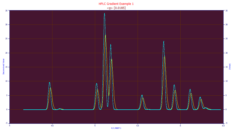
With the unwinding, there is also the convolution preprocessing that incurs a certain loss of resolution. The gradient peaks are sharper; the unwound peaks broadened. The following data set is a gradient separation where eleven peaks are apparent in the raw data (in blue). When the peaks are unwound to remove the influence of the gradient (in yellow), the widths and measure of overlap increase. The last peak changes from a local maxima peak to a hidden peak, requiring either a hidden peak algorithm, or an extra effort to place that peak.
If the above data are unwound and fitted to a Gen2HVL model as a crosscheck on the unwinding, we see a beautiful 6.3 ppm overall error in fitting the 11 peaks, but the a4 fits to 1.96, somewhat below the 1.98-2.00 or so which is typically observed with isocratic peaks, suggesting a slightly narrower Gaussian width may be needed for an optimal unwinding of the gradient.
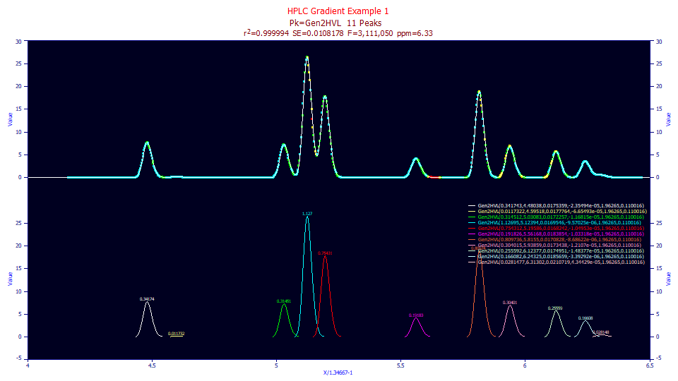
Fitted Parameters
r2 Coef Det DF Adj r2 Fit Std Err F-value ppm uVar
0.99999367 0.99999334 0.01081779 3,111,050 6.32865523
Peak Type a0 a1 a2 a3 a4 a5
1 Gen2HVL 0.34174290 4.48037660 0.01753587 -2.355e-05 1.96264980 0.11001598
2 Gen2HVL 0.01173218 4.59517993 0.01777645 -6.655e-05 1.96264980 0.11001598
3 Gen2HVL 0.31451246 5.03082657 0.01722571 -1.168e-05 1.96264980 0.11001598
4 Gen2HVL 1.12695167 5.12394331 0.01695459 -9.57e-06 1.96264980 0.11001598
5 Gen2HVL 0.75431228 5.19585957 0.01682420 -1.05e-05 1.96264980 0.11001598
6 Gen2HVL 0.19182591 5.56168467 0.01838541 -1.033e-05 1.96264980 0.11001598
7 Gen2HVL 0.80973631 5.81550059 0.01708282 -8.686e-06 1.96264980 0.11001598
8 Gen2HVL 0.30401484 5.93858754 0.01734384 -1.211e-05 1.96264980 0.11001598
9 Gen2HVL 0.25559228 6.12376906 0.01749515 -1.484e-05 1.96264980 0.11001598
10 Gen2HVL 0.16608207 6.24325486 0.01856594 -3.393e-06 1.96264980 0.11001598
11 Gen2HVL 0.02814768 6.31301715 0.02107191 4.3443e-05 1.96264980 0.11001598
The good news with gradient separations is that the two response functions do significantly offset one another, and in most instances closed form fits are not only possible, but may even be necessary to realize statistical significance in the fitting.
 |