PeakLab v1 Documentation Contents            AIST Software Home            AIST Software Support

Gen2HVL<irf> Specializations

The Gen2HVL Chromatographic Model

The twice-generalized IRF-bearing models are universal chromatographic models that will fit a variety of specializations or simplifications. The following list contains the main specializations of the Gen2HVL<ge> model:

The closed-form specializations are in blue, the non-closed form specializations are in red. All of the models are based on implementing one of more of the following simplifications:

(1) the fourth moment power of decay term is fixed at 2.0, a Gaussian. This removes the fourth moment adjustment allowing the peak to be fit with a once-generalized model.
(2) the third moment asymmetry term is fixed to 0, rendering a symmetric underlying peak. This removes the third moment adjustment allowing the peak to be fit without a generalized model.
(3) the chromatographic distortion is fixed to 0, removing all concentration-dependent tailing and fronting and allowing a non-HVL model to be fitted.
(4) the <ge> IRF is adjusted to effectively remove the 'g' half-Gaussian component, leaving only the exponential.
(5) the <ge> IRF is adjusted to effectively remove the 'e' exponential component, leaving only the half-Gaussian.

If any of these apply, you may want to fit the simpler models. The fit statistics in PeakLab's Numeric Summary will make it easy to spot parameters which are not significant in the fitting, and are probably indicative of overfitting. When a once or twice generalized chromatographic model is consistently fitting one or more parameters to insignificance (cannot test different from 0), this is welcome news. It means a simplification can probably be made.

In our experience, most analytic isocratic peaks require a once-generalized HVL model unless you are fully in the linear concentration range or have an exceptional column with no asymmetry. We have seldom seen real world data where the IRF can be treated with a single component. More often the half-Gaussian component is close to an impulse which fails to test non-zero in the fitting, but which is necessary to model the IRF decay shape.

For gradient peaks that are directly fit (the gradient is not addressed in a preprocessing step), a twice-generalized HVL model is usually needed. The nature of the gradient-introduced asymmetry almost assures the asymmetry term of a once-generalized model will be needed, and the compaction arising from the gradient will generally require the fourth moment power of decay term of a twice-generalized model. Unless you can be certain of the separations that will occur, we recommend that you use the GenHVL or Gen2HVL family of models which support nonlinear chromatographic tailing and fronting. If processing natural materials, an unexpectedly strong concentration of a given component can result in a significant measure of tailing or fronting. In modern UHPLC chromatographic separations, it doesn't take too much to shift from full linear chromatography peaks to a state where nonlinear tailing and fronting is appreciable.

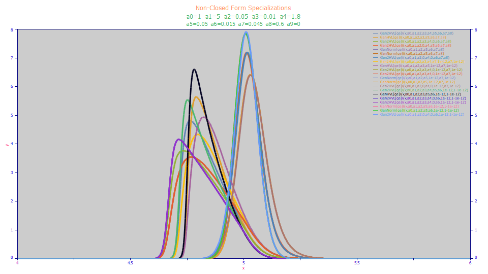
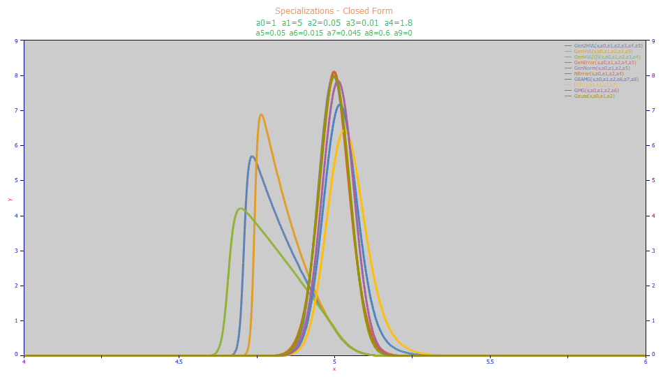
The once-generalized and twice generalized models will gracefully manage the simplifications listed above. The following are plots of non-closed form and closed-form generated data used as part of PeakLab's internal certification of the Gen2HVL model:

All of these peaks represent specializations where one or more of these five simplifications were made to just a single original set of Gen2HVL test parameters. Fits to the Gen2HVL<ge> were successful in all of the above shapes. Please note that certain programming constraints may prevent nearly flawless fits in the ppb statistical error range. For example, PeakLab does not allow one component of a two component IRF to be perfectly zeroed since the Fourier methods require a minimum IRF tau or SD for each component in the Fourier domain processing.