PeakLab v2 Documentation Contents R2N Software Home R2N Software Support
HPLC Gradient Peaks - Fitting a Deconvolution Model
Approach 2: Estimating the Convolution Model for the Gradient by Fitting a Deconvolution
PeakLab includes specialty 'deconvolution' models that can be used for discovering the gradient's system response model and parameters.
You may wish to refer to the tutorial HPLC Gradient Peaks - Fits Which Model the Gradient (Tutorial)
The basic IRF-bearing GenHVL<g> model, for example, fits a convolution of the GenHVL model with the <g> half-Gaussian response function to data. The data is assumed to be smeared and distorted by the half-Gaussian instrument response function. The parameters of the fit recover the pure model absent the IRF.
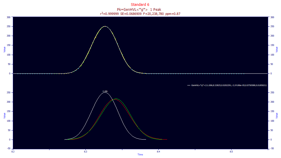
The GenHVL<*g*> model, on the other hand, does just the opposite. It fits a deconvolution of the GenHVL with the <g> half-Gaussian response function, estimating the <g> system parameter for the gradient. The gradient data is treated as deconvolved (sharpened) data as opposed to convolved (IRF-smeared) data. In this instance, the parameters of the fit recover the estimates describing the gradient as well as the estimated peak parameters had no gradient existed.
In this 'reverse' type of fitting, there is the issue of noise. As shown in plot of the zoom-in of the baseline regions on this page, the very low sample gradient HPLC concentrations produce peaks with a measure of noise, and a deconvolution only adds further noise, even with a Fourier-domain filter automatically applied.
For these reasons, you should use these gradient 'discovery' models only with single peak gradient standards for the purpose of identifying the gradient's system response function and deriving estimates for its parameters. If you use these models for any other purpose, they should be deemed purely experimental. Interestingly, since you place peaks based on the raw data, the loss of resolution from a convolution and subsequent fitting is not a factor.
The following models are available (the same IRF definitions apply):
GenHVL<*e*>, GenNLC<*e*>
GenHVL<*g*>, GenNLC<*g*>
GenHVL<*k*>, GenNLC<*k*>
GenHVL<*n*>, GenNLC<*n*>
GenHVL<*l*>, GenNLC<*l*>
GenHVL<*e2*>, GenNLC<*e2*>
GenHVL<*pe*>, GenNLC<*pe*>
GenHVL<*ge*>, GenNLC<*ge*>
The only system response models we have found to accurately describe an HPLC gradient were the <*g*> (with a retention unit SD width of approximately .015-.02) and the variable order kinetic <*k*> (with an order of 0.6-0.7 and a time constant width of 0.015-0.02 retention units).

Fitted Parameters
r2 Coef Det DF Adj r2 Fit Std Err F-value ppm uVar
0.99999913 0.99999907 0.06869090 20,238,780 0.86961687
Peak Type a0 a1 a2 a3 a4 a5
1 GenHVL<*g*> 11.0059759 8.33825080 0.02022911 -2.242e-5 0.07505876 0.01850210
A deconvolution fit can be quite effective. Fitting the GenHVL<*g*> results in an estimate of the gradient as a half-Gaussian response of 0.0185 and with a fit having less than 1 ppm unaccounted variance error.
You will note that a deconvolution fit is the reverse of an isocratic fit with an IRF. The white peak above is the gradient shape, the red peak is the unwound peak absent the influence of the gradient, and the green is the estimated pure HVL peak had an isocratic separation occurred. Note that even with a very low a3 chromatographic distortion, there is still a difference between the unwound GenHVL peak in red and unwound HVL in green.
In using this fitting method to estimate the gradient's system response function, you will probably want to use the IRF default option and set initial parameters that do not produce negative values in the deconvolutions shown which attempt to match the raw data peaks. While in fitting it is often advantageous to set starting estimates higher than the expected fit values, this is an exception since it can produce local minima fitting issues.
Also, if you choose to use the Gen2HVL and Gen2NLC versions of these "reverse IRF" models, you should use the ZDD option or Common Parameters option to lock the decay power at 2.0, 1.99, 1.98, or whatever value you have determined to best represent the Gen2HVL or Gen2NLC decay of non-gradient peaks (peaks at an isocratic start or hold). If our experience holds, the peaks in an isocratic start or hold should fit to a4 power values between 1.96-1.99. If you lock the ZDD value, be sure to unlock the Gen2HVL or Gen2NLC power parameter after these fits in order to have the fourth moment fitting available for directly fitting gradient shapes.