PeakLab v1 Documentation Contents            AIST Software Home            AIST Software Support

HPLC Gradient Peaks - Direct Closed-Form Fits

Approach 1: Direct Closed Form Fits of the Gradient Peaks which Fit the Tail Compression as a Fourth Moment Effect

The simplest approach is using a twice-generalized model such as the Gen2HVL or Gen2NLC which adjusts both the third and fourth moments of the ZDD zero distortion density. It is one of the easiest of all possible peak fits once the data have been extracted from the sloping baseline. There is nothing more to it than choosing either a Gen2HVL or Gen2NLC model to fit the peaks.

Fitting the fourth moment kurtosis using the twice generalized Gen2HVL model is covered in the tutorial: HPLC Gradient Peaks - Direct Closed Form Fits (Tutorial).

In this type of modeling, the gradient shape is fitted directly. There is no effort to model the impact or influence of the gradient. The mix of IRF and gradient effects are fit with the higher order moment adjustments in these models.

This works because any IRF that would be present in isocratic elutions, or in an isocratic hold in a gradient run, is mostly lost in the compression of the gradient. A closed form isocratic model is fit because it is not usually possible to fit an <irf> bearing isocratic model to gradient peaks. Here one is directly fitting a distorted shape where the IRF is fit together with the chromatographic model using only the higher order parameters in a Gen2NLC or Gen2HVL model to address the gradient asymmetry, the gradient compression, and the various remnants of the IRF, as well as the deviations for the theoretical zero distortion density idealities.

In gradient peaks, the IRF and gradient aren't additive; they are in opposite directions. The IRF adds tailing, the gradient removes it. The net effect is a shape that can be successfully fitted with a two higher-moment (third and fourth) generalized chromatographic model.

In fitting a Gen2HVL or Gen2NLC directly to baseline corrected gradient data, the skew or third moment a₅ parameter will probably be addressing the gradient effect far more than any deviation from a theoretical expectation of an infinite dilution density. Insofar as the kurtosis or fourth moment is generally little altered in isocratic elutions, the a₄ fourth moment parameter in a gradient peak fit will almost exclusively map the change in strength of gradient across the time of the peak's elution.

Although the Gen2HVL or Gen2HVL models are usually fitted, we can fit any one of the following closed form models:

· A twice-generalized chromatographic model which fits two higher moments in the ZDD, such as the Gen2HVL

· A specialized generalized chromatographic model which fits only the fourth moment in the ZDD, all asymmetry managed solely by the chromatographic distortion, such as GenHVL[Q]

· A generalized error model which fits a skew and asymmetry independent of the generalized chromatographic model and its ZDD, such as the GenError[m]

In this simplest strategy for gradient fitting, it is all about parameters which map as much of the orthogonality (independence, lack of correlation) of moments as possible.

Gen2HVL

The primary option uses a model such as the Gen2HVL which fits a chromatographic asymmetry (distortion) as well as an asymmetry in the ZDD. It is the latter asymmetry adjustment which makes it possible for a generalized model with a common chromatographic distortion to specialize to the HVL, the NLC, or to any other shape between or to either side with respect to skewness of the ZDD, the zero-distortion density. In the Gen2HVL there are two parameters that address skewness, a₃ which addresses the concentration-dependent distortion that produces the fronting or tailing in a chromatographic peak, and a₅ which addresses the asymmetry in the zero-distortion density that a₃ operates upon to produce the final shape. The two asymmetry parameters are necessary in isocratic peaks since the real-world zero-distortion densities will not follow either the Gaussian of the HVL, or the Giddings of the NLC models.

The fourth moment or kurtosis is addressed by the power term in the generalized error ZDD at the core of the generalized chromatographic model. This a₄ parameter will map the compression in the tails of a gradient peak. The moments 0-4 track parameters a₀-a₄. Parameter a₅, which adjusts the asymmetry of the ZDD and further adjusts the third moment is the additional parameter.

We will note that there is no reason any one of the Gen2HVL<irf> models cannot be fitted. We have not found an appreciable benefit with respect to the greater complexity of fitting a convolution integral. In directly fitting a gradient peak, most of the lack of fit will not reside in any remnant of the IRF which is still present in a gradient peak. It will rather reside in the lack of fitting of the gradient, and such can be modeled only with a deconvolution (a sharpening) of the true peak as opposed to a convolution (a broadening or smearing). If you do wish to explore such fitting, you should first try the Gen2HVL<e> model which adds a simple first order exponential IRF in a convolution integral. In order to see an improved F-statistic, indicating a model that better describes the data, you may have to determine a residual post-gradient exponential and lock that value in the IRF dialog prior to fitting.

GenHVL[Q]

This model is a simplification that assumes all asymmetry can be attributed solely to the chromatographic distortion. The GenHVL[Q] model still assumes the common chromatographic distortion is applied to a ZDD, but here there is no ZDD asymmetry. The ZDD isn't assumed to be Gaussian (it is a statistical Error density), as a more compact tail decay is being fitted, but it does assume symmetry. This is pure elegance insofar as there is one fitted parameter for each moment. Here the moments 0-4 track parameters a₀-a₄.

A GenHVL[Q] fit is identical to a Gen2HVL fit with its a₅ parameter locked at 0 (in the ZDD dialog, lock the Gen2HVL asym adjust at 1e-12 to confirm this).

If there is only a chromatographic distortion, which is to say the ZDD is a perfectly symmetric density, the GenHVL[Q] fits of gradient peaks should be identical to the Gen2HVL in goodness of fit.

Here as well there is no reason a GenHVL[Q]<irf> model cannot be fitted. If you wish to explore this, we again recommend starting with the GenHVL[Q]<e> convolution model, and locking the value of the <e> time constant at the value of the exponential IRF that you have determined to survive the gradient.

GenError[m]

This model is the reverse of the simplification in the GenHVL[Q] model. Here it is assumed that there is no a₃ chromatographic distortion, that the value is either too low to impact the peak's shape, or that such this generalized chromatographic model applicable to isocratic peaks is voided, no longer valid, in gradient peaks. This model is the generalized error density with a₁ the mean of the density instead of the underlying Gaussian. This model is actually the ZDD in the Gen2HVL model. It assumes that all of the asymmetry can be managed by the log transform in the generalized error density. In this instance, there is this same elegant mapping of one moment to one parameter. In this case, you must use the Statistical family to access this model and in this instance, the parameterization is such that a₃ addresses the tailing and thus the fourth moment, and a₄ addresses asymmetry or third moment.

A GenError[m] fit is identical to a Gen2HVL fit with its a₃ parameter locked at close to 0. To test, you will have to lock the a₃ value at 1e-12 to confirm (you can use the Set Common Parameters option for multiple peaks in a one or all data sets).

If there is no chromatographic distortion, only a statistical asymmetry, the GenError[m] fits of gradient peaks should be identical to the Gen2HVL in goodness of fit.

Inferences

In the HPLC Gradient Peaks - Direct Closed Form Fits (Tutorial), we fit eight different gradient standards. If these are modeled by these different methods discussed here and all eight of the fits averaged, we see the following:

The power of decay term is highlighted in orange in the above fit averages. The very good news is that the fourth moment, which measures the compaction or compression of the tails, is easily and accurately mapped in all of the models that fit a fourth moment tailing. There isn't much that can significantly alter the compaction of tailing that is estimated in this type of modeling. The power of 2.13 indicates an appreciable compression.

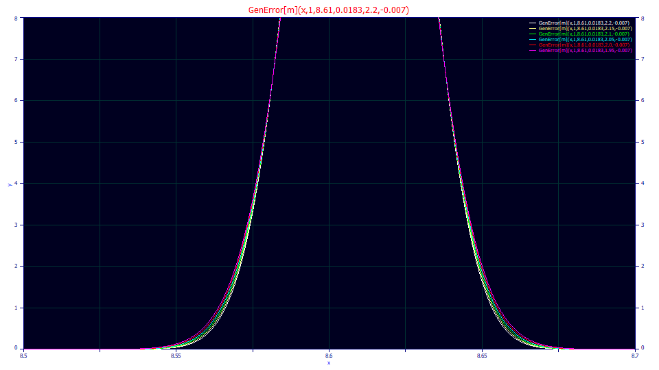
Above is a plot using these averages and varying the power of decay from 1.95 to 2.20, from a typical lower bound for an isocratic peak to a typical upper bound for gradient peaks. The difference in the kurtosis or fourth moment is mostly in the tails. A peak can appear Gaussian to the eye, but it isn't easy to visualize the thickness of the tails and errors which occur near the baseline of peaks.

More challenging is that both of the third moment factors, the chromatographic distortion a₃ in the Gen2HVL and GenHVL[Q] models, and the statistical asymmetry in the a₅ of the Gen2HVL and the a₄ of the GenError[m] models, are very small, but neither can be treated as insignificant.

We can infer that a fourth moment term is essential (comparing the Gaussian with the NError model). We can then infer than a third moment term is essential as well (comparing the NError with the GenHVL[Q] and GenError[m] models). We can also infer that the chromatographic distortion of the GenHVL[Q] probably better describes the skewness than the statistical asymmetry in the GenError[m], if only a single skewness term is fitted.

If we add the chromatographic distortion to the GenError[m] to get the Gen2HVL, the F-stat improves slightly suggesting a better model. If we add the statistical asymmetry to the GenHVL[Q], again to get the Gen2HVL, the F-statistic drops slightly suggesting the addition doesn't quite produce a better description of the data.

Because the gradient is not modeled in this type of fit, only the higher moments of the peak resulting from the gradient, the 10-20 ppm unaccounted variance may be about the best you can realize from this simplest form of gradient peak modeling.

As you will note from the averages of the parameters above, the second and fourth moment terms are readily modeled. It is with the skew that the estimation differences rest. Also, bear in the mind that the significance test statistically checks to see if an estimated value is different from zero. If you see a failed significance on the statistical skew, it may be that the peak is too close to symmetric for this parameter to estimate a value for a statistical asymmetry. Unlike that which you see on the a₀-a₃ parameters in a chromatographic fit, a failed significance on the a₅ in the Gen2HVL may be fine since a zero a₅ is the ideal. If you consistently see near zero values for the a₅ in the Gen2HVL, you can fit the GenHVL[Q] model, or simply lock the Gen2HVL's asymmetry at a value near 0 (we recommend 1e-12).

We mentioned that an IRF can optionally be fitted in the Gen2HVL and GenHVL[Q] models, and we suggested that the simple <e> exponential IRF be the primary one that is explored, since we know a portion of the exponential of the isocratic IRF can survive the gradient. The table below again includes the averages from eight separate gradient peak fits.

There is an improvement in the overall error, but the F-statistic suggests little modeling power benefit, and the price is a steep one for the tiny gain. The <e> models are integral fits that often require minutes instead of seconds.

Modeling HPLC Gradient Peak Shapes with a Gen2HVL Model

In directly fitting HPLC gradient shapes, these are the key points to keep in mind:

(1) For peaks that occur within the gradient, while the mobile phase is increasing in strength during the peak's actual elution, the gradient will probably mask most of the instrumental distortions. If you attempt to fit these peaks to an <irf> model, the goodness of fit may actually be poorer. In this direct approach, any remnant IRF is fit using the higher moments of the closed-form model.

(2) For peaks that occur within an isocratic start or later hold, an <irf> fit should be possible, but to the extent the IRF is impacted by the strength of the mobile phase, the system IRF may be different in these two different holds. You cannot use a Gen2HVL or Gen2NLC fit to model the isocratic peaks to a high accuracy. You will need a GenHVL<irf> or GenNLC<irf> model.

(3) The peaks that elute during the gradient may deceptively appear as symmetric Gaussians, but they will actually have a unique shape which is a combination of a compression of a chromatographic peak shape in time arising from the gradient's influence on the peak's elution, and the actual tailing arising from the same kinetic and probabilistic IRF effects which arise in an isocratic separation. Such a peak will have its own unique density, and there will be a net compaction of the tails.

(4) Since the gradient compression alters the kurtosis or fourth moment, the 'thinness' or 'fatness' of the tails, you cannot fit a GenHVL or GenNLC model which adjusts only the third moment or skew, but largely retains the overall rate of decay of the tails. You must fit a twice-generalized model, such as the Gen2HVL or Gen2NLC where the fourth moment, the kurtosis is also adjusted.

(5) An analytic peak in an isocratic elution will typically have a fourth moment power term in the Gen2 models just under 2.0. Typical fitted values are 1.96-1.99. As a consequence of the compression arising from the gradient, this term will be higher than 2.0 for gradient peaks, and should be an indirect measure of the change in gradient across the time of elution of that peak. You should expect to see values in the vicinity of 2.05-2.2 for this fourth moment term which describes the power of the decay. A tail decay in the Gen2HVL of 2.0 is a perfect Gaussian, a statistical kurtosis of 3.0.

(6) The kinetics in the GenNLC and Gen2NLC models are based on the first order kinetics of an assumed Giddings zero-distortion density. Since a Giddings density will not exist in a gradient shape, you may wish to reserve the NLC-based models for the second and third approaches which model the gradient and fit an unwound shape where the GenNLC and its Gidding assumption will be valid.

(7) In attempting to realize the finest possible fits of gradient HPLC peaks, the most challenging aspect of such will likely be the baseline subtraction. You will probably see the best results from a manual baseline subtraction using the non-parametric linear model. Using this method, you can manually isolate the baseline points on the gradient slope, but even with such careful attention, very small peaks that barely rise above a sharply changing baseline may be close to impossible to fit accurately.

(8) For close to full accuracy fits, the second and third approaches which model the gradient will be needed. PeakLab offers an effective procedure for deconvolving the gradient (and its embedded IRF) from gradient peaks, an approximation of the isocratic peak shape that would have existed had there not been a changing gradient during the peak's elution. Once a model for the gradient has been determined, it is a simple matter to unwind the gradient in the IRF Deconvolution procedure and fit isocratic models.

Interpreting the Parameters of a Gen2HVL or Gen2NLC Direct Fit of a Gradient Peak

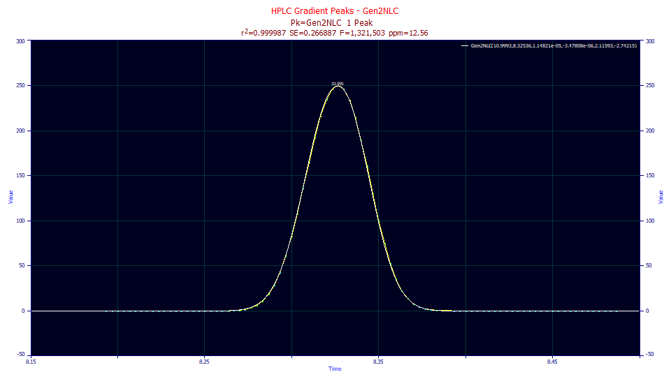
The above peak is a gradient HPLC standard. Here the only adjustment was a dead time correction and the baseline adjustment for the sloping gradient. The raw data for this peak consisted of less than 100 data points. The fit was very good, 12.5 ppm unaccounted variance. In this example, we show the fitted results for both the Gen2HVL and Gen2NLC using the Equivalent Parameters option in the Numeric Summary.

Fitted Parameters

r² Coef Det        DF Adj r²          Fit Std Err        F-value            ppm uVar

0.99998744         0.99998652         0.26688742         1,321,500          12.5613253

 Peak        Type                 a0                a1                a2                a3                a4                a5    

    1        Gen2NLC        10.9993050        8.32535900        1.1482e-5         -3.478e-6         2.11592580        -2.7421515  

Equivalent Parameters

 Peak        Type                 a0                a1                a2                a3                a4                a5    

    1        Gen2HVL        10.9993050        8.32535900        0.01382700        -3.478e-6         2.11592580        -0.0045542  

Parameter Statistics

Peak 1 Gen2NLC

 Parameter           Value             Std Error         t-value           95% Conf Lo        95% Conf Hi

         Area        10.9993050        0.00488967        2249.49777        10.9895797         11.0090304

       Center        8.32535900        0.00013753        60535.1654        8.32508546         8.32563254

        Width        1.1482e-5         1.5438e-7         74.3757530        1.1175e-5          1.1789e-5 

     Distortn        -3.478e-6         6.601e-7          -5.2690547        -4.791e-6          -2.165e-6 

      Q-power        2.11592580        0.00334057        633.402122        2.10928154         2.12257006

      NLCasym        -2.7421515        1.42988538        -1.9177422        -5.5861360         0.10183304

HPLC gradient peaks produce very high kinetic rates (very low a₂ time constants in the Gen2NLC), or very small widths (Gaussian SD values in the Gen2HVL), In this same data, the a₃ chromatographic distortion fits with an exceptionally low magnitude fronting (negative a₃).

The a₄ value is 2.11, well above the 2.0 power of a Gaussian decay and the 1.96-1.99 typically found with isocratic peaks. The tails are strongly 'thinned' by the compression. Another way to state this is that the tails are more 'compact' than a Gaussian. Since the kurtosis almost exclusively changes with the rate of change of the gradient during the peak's elution, the a₄ parameter will measure the power of the gradient for a given a₂ peak width. If a solute elutes with a higher a₂ width, you may see a corresponding reduction in the a₄ of the peak.

In an isocratic fit, the a₅ asymmetry in the ZDD measures the deviation from the ideality of a Gaussian (a₅=0 in both the Gen2HVL and Gen2NLC) or the Giddings (a₅=0.5 in the Gen2NLC). The negative a₅ ZDD asymmetry in this fit is measuring the net asymmetry between the gradient and the IRF. An isocratic peak would be expected to have a ZDD asymmetry of about 1.0-1.5 in the GenNLC model, a value higher than the 0.5 of the theoretical NLC. The -2.74 a₅ represents a strong left skew that is also indicative of the strength of the gradient. Such a negative value represents an offset of nearly all of the IRF and results in a fronted (negative, left skewed) ZDD asymmetry, something rarely observed in accurate fits of isocratic peaks.

If you look at the absolute value of the t-value in the parameter statistics for the fit in the plot, you will see that the a₁ center is most accurately determined, the a₀ area is next, and the tail compression parameter, a₄, is actually ahead of the a₂ peak width with respect to this accuracy of determination. The a₃ chromatographic distortion is only weakly estimated, and the a₅ ZDD asymmetry doesn't quite fit as statistically significant (different from zero). If you are fitting Gen2NLC or Gen2HVL models to gradient HPLC peaks, use these parameter statistics generously with respect to inferences.

The problem with using a₅ as an estimate of the gradient is that the ZDD asymmetry changes the density that the a₃ chromatographic distortion operates upon. When the a₃ is strong, small changes in the ZDD result in large changes in the chromatographic shape. When a₃ is close to zero, as is the case here, the density is much less altered by a₃. Again, please note that the a₅ parameter is the weakest of the parameters estimated. In contrast, note how strongly the 2.11 a₄ parameter is estimated. The a₄ parameter should be used as the estimate of the gradient strength.

We also note that we have observed that the widths of gradient peaks can impact the a₄ power of decay. Peaks elute generally close to constant widths within a gradient, but there may be small differences where peaks with a higher a₂ width tend to have a lower a₄ thinning of the tails. If you see two peaks with differing a₄, this should not automatically imply differing gradient strengths at these points in the gradient program. Check the a₂ widths. If the two peaks have very close to the same widths, only then should they be expected to have the same a₄ thinning of the tails with a constant gradient.

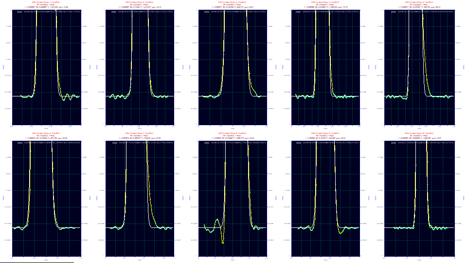
The above represents a zoomed-in baseline region of ten different gradient peak fits. The Gen2NLC or Gen2HVL will not manage the tiny bit of IRF that is left in the last portion of the decay on certain of the samples, and obviously none of the baseline oscillations. However so, the fits are very good ones, and the parameters will be determined with approximately the accuracy suggested in the confidence bands.

When fitting a gradient peak shape to a twice-generalized chromatographic model, the shape will not generally be modeled with the fit errors following a Gaussian or normal distribution, especially since the gradient itself is not fitted. In fact, this non-Gaussian error density is often true of very high accuracy chromatographic modeling in general. When only a few ppm error remain within a fit, the errors associated with that tiny measure of unaccounted variance are unlikely to be normally distributed. This does mean that the confidence statistics for parameters may be wider than the intervals reported which are based on this normal assumption.

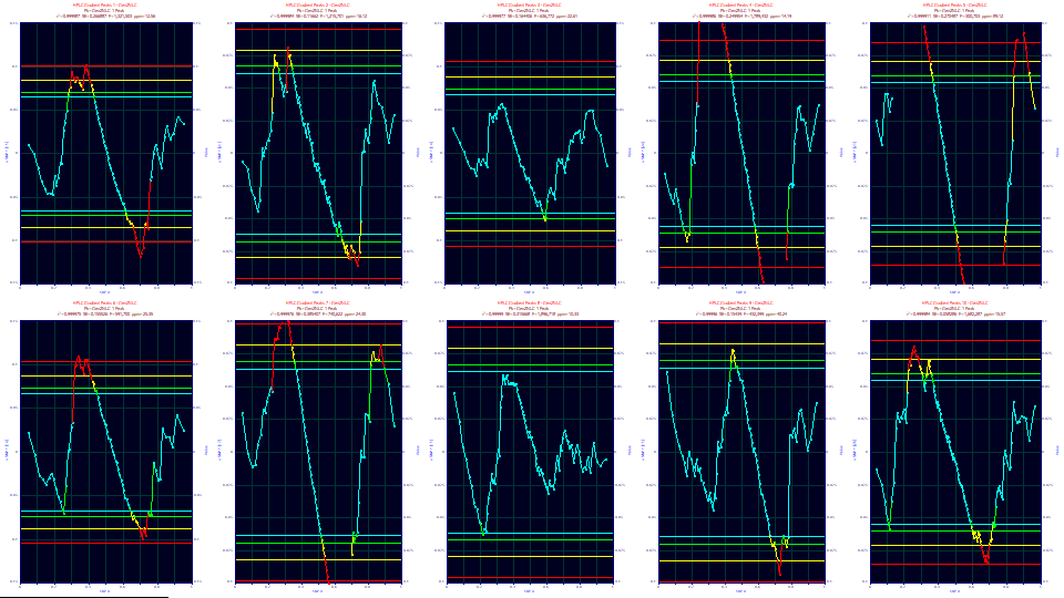
Before adopting the confidence statistics as valid, you will want to be certain the errors in the fit are normally distributed. You can use the SNP plot within the Residuals option. For these ten fits, only the third and eighth data sets test as having normally distributed errors. For the others, the actual parameter confidence bands about the parameters will be somewhat wider. Fortunately, on very high accuracy fits, the confidence bands will tend to be small on the parameters strongly estimated. If you are interested in the 95% confidence band around the a₄ fourth moment parameter which estimates the strength of the gradient, you should use this SNP test to assess the statistical validity of those intervals.

Guidance for Baseline Subtraction

The automated baseline subtraction routines will likely require the SD Variation algorithm for gradient peaks. You will probably have to use high values for the threshold option, although the baseline % option should find close to that percent of baseline points. If you find that very small peaks are being assigned as baseline, you will need to manually assign the baseline points.

In the baseline procedure, the manual sectioning mode will be selected in the graph's toolbar, but you can change to a zoom-in mode if needed to narrow the zone of the data for better detail, and then return to this sectioning mode to complete the selection of baseline points.

To manually assign points as baseline the easiest method is to place the mouse to the far right of the data, click and hold the mouse sliding left across the data. All of the points will turn yellow and be assigned as baseline. Now place the mouse cursor at the beginning of each peak, click and hold sliding right to assign such points as peak data, releasing the mouse where you deem the baseline to have resumed. The peak points will show as grayed, as non-baseline.

A baseline is fit to a model, and you will almost certainly need the Non-Parm Linear, the non-parametric linear algorithm. The NP n is the count of points used in the sliding linear fit across the data. To have all of the points assigned as baseline to be zero, you must check the Zero Baseline points post-processing option. This option is useful for removing all features from the data you do not wish to subsequently fit.

Fitting a Gaussian vs Gen2HVL

Because a gradient peak visually looks symmetric, you may be tempted to fit such data to a simple Gaussian model.

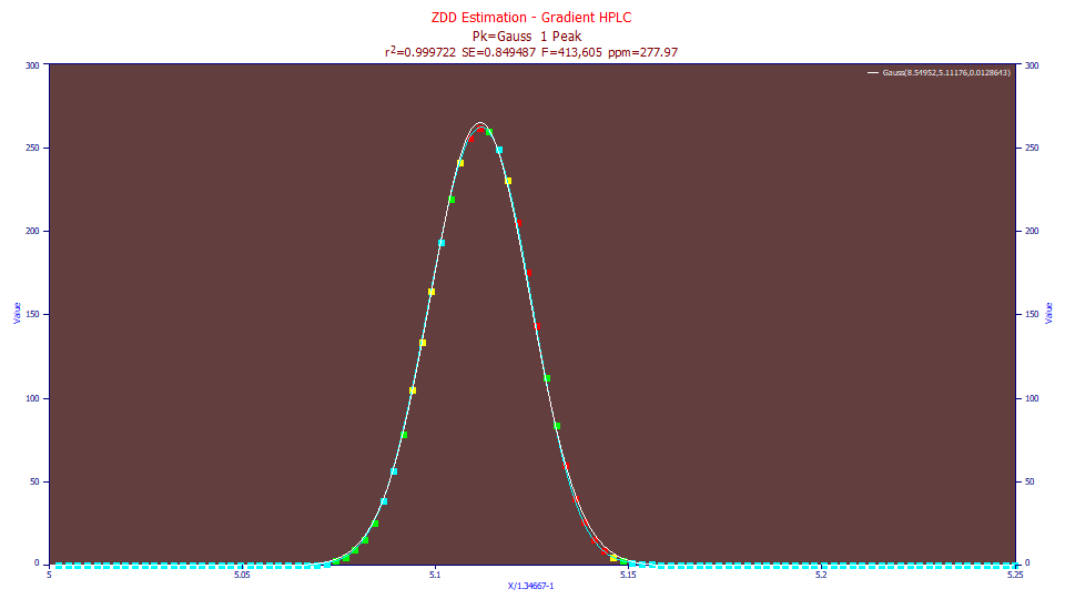
We have an error of 278 ppm unaccounted variance. We used the Points toolbar option to make the data points larger and we changed the connected lines to a cubic spline for better visualization of the fit. The gradient peak is not a Gaussian. Close to the baseline, both the rise and decay are sharper. If you look closely, the gradient peak is also slightly fronted, more mass to the left of the apex, than to the right.

The Gen2HVL model is the model we recommend for the direct fitting of gradient shapes. If we fit the Gen2HVL model to this same data:

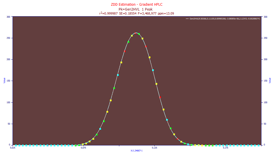
Fitted Parameters

r² Coef Det        DF Adj r²          Fit Std Err        F-value            ppm uVar

0.99998691         0.99998657         0.18553950         3,468,977          13.0872605

 Peak        Type                 a0                a1                a2                a3                a4                a5    

    1        Gen2HVL        8.50365871        5.11104926        0.00985306        -3.081e-6         2.12343112        -0.0028867  

Measured Values

 Peak        Type            Amplitude          Center             FWHM             Asym50           FW Base            Asym10    

    1        Gen2HVL        261.553899        5.11223440        0.03089580        0.93750642        0.05963298        0.94365942  

 Peak        Type              Area             % Area             Mean             StdDev           Skewness          Kurtosis   

    1        Gen2HVL        8.50365871        100.000000        5.11162177        0.01261704        -0.0347217        2.88769498  

Chromatographic Analysis

 Peak        Type             Nmoment          NGauss           FW Base            Asym10          Resolution         Retention  

    1        Gen2HVL        1.6414e+5         1.5182e+5         0.05963298        0.94365942                          5.11104926  

As in the prior example, the fit is much improved, the error 13.1 ppm. Because the gradient is not fitted, we have seldom seen direct fits to the gradient shape which were less than 10 ppm error. As you will note from the plot, the cubic spline through the data and the Gen2HVL fit visually overlap, or at least far more than does the Gaussian fit.

The a₃ chromatographic distortion again fits to near 0, and slightly fronted. The asymmetry of the ZDD in a₅ is again negative. It is a₄, the power of decay, which maps the difference in the power of the tails which distinguishes a gradient peak. Its value of 2.12 is close to typical of the value we expect to see in a gradient peak's compression or 'thinning' of the tails in this fourth moment.

Note also the third and fourth moments of the Gen2HVL model. With respect to this direct fitting of gradient shapes, you may find it convenient to use the third and fourth moments instead of the a₃-a₅ parameter values. Note that the skewness gives an estimate of the fronting, and the kurtosis an estimate of the gradient compression. At 2.89, the kurtosis is well below the 3.0 of the Gaussian.

We will note that the analytic and deconvolved moments of the Gen2HVL in the Numeric Summary only have a meaning in non-gradient fits. The plate values in the Chromatographic Analysis section of the Numeric Summary, however, will be valid.

A Composite of IRF and Gradient Effects

Please remember that the gradient peak shape has two different response functions. One dilates the chromatographic peak shape with an IRF convolution, a further broadening, the other compresses the shape with a gradient deconvolution, a sharpening. The two processes offset to a significant degree. The composite shape may have very little chromatographic a₃ distortion, and only a very small a₅ asymmetry, but there is no reason to believe that the two different response functions fully cancel one another. Indeed, one would expect a measure of each to survive, which is exactly what we have found in a large number of gradient fits.

Fitting Real-World Gradient Separations with the Gen2HVL Model

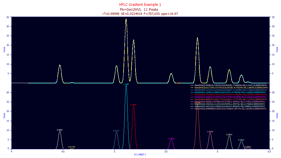
The challenge with real world data will rest mainly with this same baseline separation accuracy we previously discussed. Here we have a gradient separation that consists of 11 peaks. We achieve a high goodness of fit, 19.97 ppm with the Gen2HVL, holding the a₅ asymmetry, which we expected to be very small, shared across all peaks:

Fitted Parameters

r² Coef Det        DF Adj r²          Fit Std Err        F-value            ppm uVar

0.99998003         0.99997875         0.02249190         797,655            19.9672139

 Peak        Type                 a0                a1               a2               a3               a4               a5   

    1        Gen2HVL        0.34091495        4.46733976        0.01403394        -7.04e-6          2.13141483        0.00092294  

    2        Gen2HVL        0.01172760        4.57733642        0.01343383        -8.755e-5         1.68545469        0.00092294  

    3        Gen2HVL        0.31371428        5.01704651        0.01348541        -5.735e-6         2.11955707        0.00092294  

    4        Gen2HVL        1.12483972        5.10991280        0.01312741        -6.749e-6         2.11095833        0.00092294  

    5        Gen2HVL        0.75648570        5.18167106        0.01304693        -8.782e-6         2.09489066        0.00092294  

    6        Gen2HVL        0.19061515        5.54842557        0.01474978        2.0427e-6         2.10356142        0.00092294  

    7        Gen2HVL        0.80807866        5.80177019        0.01328413        -3.771e-6         2.11042634        0.00092294  

    8        Gen2HVL        0.30366033        5.92588263        0.01375380        1.5359e-6         2.14280620        0.00092294  

    9        Gen2HVL        0.25523009        6.11133770        0.01403757        1.2947e-6         2.17368532        0.00092294  

   10        Gen2HVL        0.16312346        6.22954732        0.01461902        4.9037e-6         2.09691868        0.00092294  

   11        Gen2HVL        0.03099084        6.30239611        0.01724678        9.1948e-5         1.62392201        0.00092294  

Two of the peaks have very small areas. These fit very poorly with respect to a₄. You should not expect to fit accurate higher moments on such peaks. You can fit and ignore these very low area peaks, they can be zeroed in the baseline subtraction, or they can be omitted from the placed peaks and ignored in the fitting. Apart from these tiny peaks, the nine with appreciable areas fit to an average a₄=2.12 with a range of 2.094-2.173.

When you see a failed significance on an asymmetry parameter, as with the a₅ in these fits, it only means the parameter cannot be deemed statistically different from zero. In this instance, it is not a matter of an overspecified fit, but of a ZDD whose asymmetry cannot be seen as anything other than symmetric. When this occurs you can usually fit the GenHVL[Q] model (which enforces zero ZDD asymmetry) and see the same results.

For very small peaks, discrepancies may well be baseline related. It is very hard to baseline correct a tiny peak on a sharply sloping baseline and close to impossible to make a clean baseline correction if two peaks overlap somewhat very close to that point in a gradient separation where the baseline experiences a reversal in signal direction.