PeakLab v2 Documentation Contents R2N Software Home R2N Software Support
HPLC Gradient Peaks - Fitting the Unwound Data
Approach 3: Unwinding the Gradient and Fitting a Once-Generalized Model with or without an IRF
If the gradient is perceived as a non-linear transform that compresses a peak, one can use the program's convolution/deconvolution engine to seek to unwind or undo the gradient, approximating the peak that would exist if the gradient had not occurred. Unlike the IRF deconvolution, where one seeks to remove a distortion to recover the true peak, here we seek to recover the true peak by adding back that which occurred within the gradient. In other words, we treat the gradient process as a deconvolution which narrows the peak, and we apply a convolution to restore the original width and shape of the peak. We treat the gradient process as a deconvolution which is undone by a subsequent convolution with an IRF which represents its system response function.
You may wish to refer to the tutorial: HPLC Gradient Peaks - Fitting Unwound Data (Tutorial)
In the spirit of allowing the data to reveal the nature of the system IRF altering it, we can take the simple approach of convolving different IRFs to see if a peak shape can be restored which can be more accurately fitted with an isocratic model. We can make the inference that the better an isocratic model is fitted, the closer we are to the IRF or system model that represents the gradient process.
If the gradient process is a purely linear one, we can use a zero order kinetic model to restore the peak shape. If the gradient process is first order, we can use an order 1 kinetic model. We can convolve any order kinetic model we wish. We can also fit a probabilisitic IRF. If we assume the gradient process is akin that of a one-sided Gaussian deconvolution, we can restore the original peak shape by convolving a simple half-Gaussian response function.

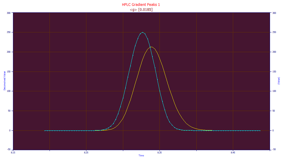
In this example, we apply a simple one-parameter Gaussian convolution data to the first data set (in blue above), the one we directly fit with the Gen2NLC model and realized a 12.5 ppm unaccounted variance. If this fit of the convolved data (the yellow curve) is significantly improved, we can assume we have unwound at least a portion of the gradient without introducing more harm than benefit. In fairness, convolution does smooth data, so we will see a modest improvement from this noise reduction, but only so long as the new shape is at least as applicable as the original to the model used in the fitting.

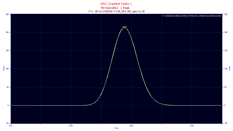
The half-Gaussian convolved data fits to an astonishing 0.28 ppm unaccounted variance, a 50x reduction in the squared error.
Fitted Parameters
r2 Coef Det DF Adj r2 Fit Std Err F-value ppm uVar
0.99999972 0.99999969 0.03589583 58,284,780 0.28480840
Peak Type a0 a1 a2 a3 a4 a5
1 Gen2NLC 10.9961570 8.33755300 2.4757e-5 -1.98e-5 2.00155019 30.1860459
Equivalent Parameters
Peak Type a0 a1 a2 a3 a4 a5
1 Gen2HVL 10.9961570 8.33755300 0.02031824 -1.98e-5 2.00155019 0.07356203
Parameter Statistics
Peak 1 Gen2NLC
Parameter Value Std Error t-value 95% Conf Lo 95% Conf Hi
Area 10.9961570 0.00072634 15139.1556 10.9947124 10.9976017
Center 8.33755300 4.0391e-5 2.0642e+5 8.33747266 8.33763333
Width 2.4757e-5 4.543e-8 544.959992 2.4667e-5 2.4848e-5
Distortn -1.98e-5 3.7678e-7 -52.540847 -2.055e-5 -1.905e-5
Q-power 2.00155019 0.00052882 3784.91919 2.00049839 2.00260200
NLCasym 30.1860459 0.21616022 139.646626 29.7561119 30.6159799
The a4 of the Gen2NLC fit is 2.002, essentially a pure Gaussian decay. Unlike the prior fit where the gradient was not unwound, here all of the parameters have strong significance. If you can identify and quantify the gradient's response function, as we did here, you can fit a GenNLC or GenHVL to the convolved data:
Fitted Parameters
r2 Coef Det DF Adj r2 Fit Std Err F-value ppm uVar
0.99999969 0.99999967 0.03749380 66,778,129 0.31447412
Peak Type a0 a1 a2 a3 a4
1 GenNLC 10.9967995 8.33749378 2.4886e-5 -2.046e-5 30.4568072
Equivalent Parameters
Peak Type a0 a1 a2 a3 a4
1 GenHVL 10.9967995 8.33749378 0.02037084 -2.046e-5 0.07441454
Parameter Statistics
Peak 1 GenNLC
Parameter Value Std Error t-value 95% Conf Lo 95% Conf Hi
Area 10.9967995 0.00072330 15203.5459 10.9953611 10.9982379
Center 8.33749378 3.6714e-5 2.2709e+5 8.33742077 8.33756678
Width 2.4886e-5 1.2767e-8 1949.29874 2.486e-5 2.4911e-5
Distortn -2.046e-5 3.1904e-7 -64.124470 -2.109e-5 -1.982e-5
NLCasym 30.4568072 0.20405363 149.258834 30.0510241 30.8625902
Here we have a higher F-statistic in the simper model. A F-statistic represents a model's capacity to represent the data properly accounting the number of parameters thrown at the fitting problem.
Fitting an GenHVL-based vs GenNLC-based Model for HPLC Gradient Peaks
The GenHVL model fits an a2 deconvolved Gaussian SD and an a4 generalized normal asymmetry at infinite dilution. The GenNLC fits an a2 kinetic width, the time constant of first order Giddings kinetics, and an a4 asymmetry indexed to both the Gaussian(HVL) at a4=0 and to the Giddings(NLC) at a4=0.5.
Since the Equivalent Parameters section of the Numeric Summary offers the parameters for both, you may wish to fit whichever model offers the confidence statistics you are most interested in. For fitting single peaks, there is no difference between the fit of these models. We mention elsewhere the value of selecting a kinetic or probabilistic generalized model based on an asymmetry parameter shared across peaks. Whereas this can make small differences in non-gradient analytic peaks, for gradient peaks the differences are negligible because of the low a3 chromatographic distortion.
Drawbacks of a Convolution Preprocessing
There is the obvious issue of loss of resolution. In the 11 peak example, all 11 peaks are clear, even if several are not fully baseline resolved.

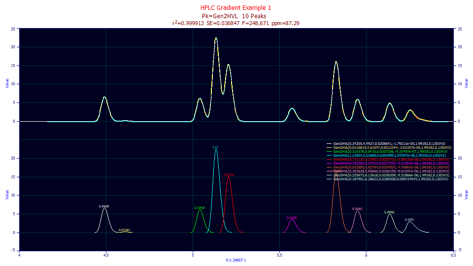
If we apply the half-Gaussian convolution to undo the gradient and fit the 11-peak data set, there are just 10 local maxima peaks which fit to a higher 87 ppm unaccounted variance. The original tenth and eleventh peaks fit as a single peak of an asymmetric shape.
Fitted Parameters
r2 Coef Det DF Adj r2 Fit Std Err F-value ppm uVar
0.99991271 0.99990859 0.03684701 248,671 87.2855663
Peak Type a0 a1 a2 a3 a4 a5
1 Gen2HVL 0.34204975 4.49269628 0.02086406 -1.792e-5 1.99181957 0.13034307
2 Gen2HVL 0.01166148 4.61046668 0.02123436 -3.016e-5 1.99181957 0.13034307
3 Gen2HVL 0.31537769 5.04350031 0.02072665 -9.335e-7 1.99181957 0.13034307
4 Gen2HVL 1.13003945 5.13668427 0.02049991 1.936e-6 1.99181957 0.13034307
5 Gen2HVL 0.75112499 5.20832806 0.02024335 -2.882e-6 1.99181957 0.13034307
6 Gen2HVL 0.19236483 5.57414105 0.02173971 -3.214e-6 1.99181957 0.13034307
7 Gen2HVL 0.81058549 5.82764475 0.02048346 -4.459e-6 1.99181957 0.13034307
8 Gen2HVL 0.30362755 5.95064910 0.02061090 -9.616e-6 1.99181957 0.13034307
9 Gen2HVL 0.25567534 6.13617861 0.02083078 -9.519e-6 1.99181957 0.13034307
10 Gen2HVL 0.18790095 6.28622363 0.02883085 0.00043404 1.99181957 0.13034307
When applying the convolution and subsequently fitting the unwound data, we are also giving up the improved resolution derived from the gradient. While the a4 parameter fits very close to 2, the loss of resolution means that peak 11 must be fitted as a hidden peak where it was a straightforward matter to fit the Gen2HVL or Gen2NLC directly to the original data.
Note that a Gen2HVL or Gen2NLC fit to gradient data can uncover hidden peaks as evident by both a2 and a3 in this example.