PeakLab v1 Documentation Contents AIST Software Home AIST Software Support
HPLC Gradient Peaks - Fits Which Model the Gradient (Tutorial)
In this example, we will fit HPLC gradient peak data to a high degree of modeling accuracy. To do so we use a new fitting procedure, deconvolution fitting, which will fit an estimate for the system gradient in the model.
In the HPLC Gradient Peaks - Direct Closed Form Fits first tutorial for gradient peak fitting, we estimated the isocratic (continuous mobile phase) <ge> IRF, the instrument/system response consisting of an area weighted half-Gaussian and first order (exponential ) as [g=0.01099, e= 0.0161, areafrac= 0.625]. We also used IRF Deconvolution to ascertain that about .006 of the .016 of the exponential survived the gradient.
We also established for eight gradient peaks, an average unaccounted variance of 16.65 ppm and 1.259M in the Gen2HVL fits which directly fit the upper moments of the peaks as eluted. Any approach to incorporate the gradient in the modeling will have to improve upon these already excellent goodness of fit values. In this tutorial we will be fitting the same eight gradient peaks.
In the HPLC Gradient Peak Fitting topic, we also report the results of fitting a convolution model to capture the remains of the exponential component of the IRF that exists in the presence of a gradient elution. In that summary, we report 13.74 ppm as the average goodness of fit for these same eight fits using a Gen2HVL<e> convolution model.
In fitting individual high S/N IC peaks to GenHVL<irf> isocratic models, all with two-component IRFs, across a large array of system variables, we have a benchmark goodness of fit which averages 2.67 unaccounted variance across 144 different data sets. We will use such as a target in this tutorial. We will seek to fit the eight gradient peaks to this 2.7 ppm average unaccounted variance.
![]() Use the File menu's Open item and select the file HPLCGradientStd02.pfd from the
program's installed default data directory (\PeakLab\Data). The file contains eight data sets, each a
baseline-corrected data set from a single standard which elutes during the gradient.
Use the File menu's Open item and select the file HPLCGradientStd02.pfd from the
program's installed default data directory (\PeakLab\Data). The file contains eight data sets, each a
baseline-corrected data set from a single standard which elutes during the gradient.
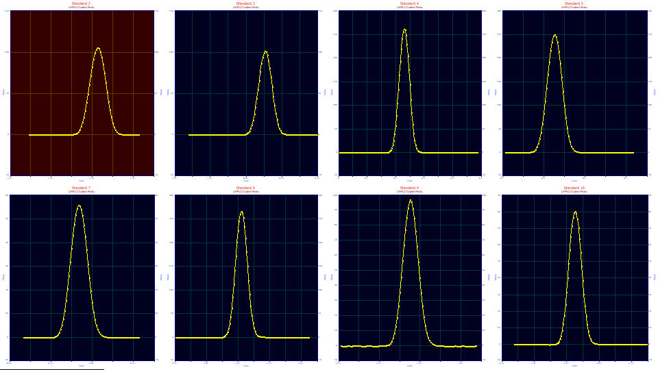
Modeling the Gradient's Influence on a Peak
If we assume a gradient elution doesn't make the IRF and ZDD distortion effects vanish, but rather adds another, a reverse effect, a directional compression which occurs as the peak elutes across a finite time, we can treat the overall fitting problem as the mathematical mix of a convolution and deconvolution applied to the isocratic peak model.
Since we have observed that much of the IRF does not survive the compression, we will begin with the simplest approach where, as in the first tutorial's approach of directly fitting closed form models, we will attempt to achieve effective fits without the convolution portion of the modeling, that which addresses the IRF. We will still fit the a3 chromatographic distortion and the additional asymmetry parameter that adjusts the third moment so that a generalized model can exactly replicate the HVL, NLC, and other ZDD asymmetry-based differences, but instead of fitting a fourth moment term, we will seek to 'unwind' the gradient using a deconvolution fitting which internally removes the compression of the gradient in the actual model.
In this approach, we must identify the model that describes how the the changing hydrophilic-hydrophobic gradient impacts a peak, and we must have a method that accurately estimates its parameter(s). Although the gradients are usually linear by concentration of the various mobile phase compounds, the influence on a peak will not be linear; one cannot simply linearly dilate or inflate the x-scale of the gradient peak to unwind the influence of the gradient and regenerate the isocratic shape. A zero order kinetic model convolution will unwind or undo a linear compression. In practice, the models for unwinding or undoing the impact of a gradient will be nonlinear, and we have found a simple half-Gaussian, as well as kinetic decay of a fractional order between 0.5 and 0.8, to be viable models.
Fitting a Once-Generalized Model with a Gradient Deconvolution in the Model
In order to unwind a gradient, one only needs the convolution model and its estimated parameters. The convolution can be easily applied to the incoming data in the IRF Deconvolution procedure and the data subsequently fitted using any of the program's isocratic models. A separate step of unwinding the gradient by the application of a convolution produces additional broadening which will reduce the resolution of the peaks, possibly so much that a local maxima peak becomes hidden in the rise of decay of an adjacent and larger peak. We will cover this approach in the third of these gradient peak tutorials.
The ideal would be a non-linear fitting approach which not only estimates the IRF for the gradient but makes this two-step process unnecessary, avoiding this issue of diminished resolution.
To accomplish this, the model must treat the gradient as an IRF which is deconvolved rather than convolved. In general, an IRF is used in a convolution model. The IRF smears a pure data shape; a narrower peak is broadened by the IRF to produce the observed data peak. In a deconvolution model, the IRF is a system model that assumes the true peak (the peak absent the gradient) is actually wider, and it has been narrowed by the influence of the IRF, the gradient. In the traditional convolution fitting, the IRF is treated as a factor of additional distortion. In a deconvolution fit, the IRF is treated as a factor that removes rather than adds broadening.
In this approach for fitting gradient peaks, we fit a model of an 'unwound' wider shape deconvolved with the IRF of the gradient to produce the observed peak. These are challenging fits since deconvolution always adds noise to the system (a convolution smoothes data and reduces noise). If this loss in S/N is effectively managed, however, this can be a complete one-step solution for fitting gradient peaks. One is not actually fitting unwound data with its corresponding broadening or loss of resolution since all is internal to the model. This approach, like the direct fitting of closed form models covered in the first tutorial, allows for the gradient to be fitted and estimated on a per-peak basis. This estimates the strength of gradient each peak sees, and it is an effective way to check for constancy in the gradient. The process of fitting deconvolution models to gradient peaks is covered in the HPLC Gradient Peaks topic.
Even though one is fitting a deconvolution rather than a convolution, we are still addressing a method that requires the same discrete Fourier domain processing (except in reverse). Fitting a deconvolution model has the same drawback in fitting speed as fitting a convolution integral. The Fourier methods, while slower, are still much faster than fitting an integral directly, but they will also be appreciably slower than fitting a closed form model with full analytic partial derivatives.
Fitting the Gradient using the GenHVL<*g*> Deconvolution Model
PeakLab includes a small subset of specialty models for directly fitting an IRF model for the gradient. A deconvolution model (as opposed to the more commonly used convolution model) is represented with an <*irf*> suffix. Here we will fit the GenHVL<*g*> model to derive the system parameters for unwinding the gradient.
Click the Local Maxima Peaks button.
Leave the settings exactly as they were set in the Gen2HVL fit, except change the peak family to the Chromatography w/IRF models and select the model to the GenHVL<*g*> deconvolution model:
Peak Detection
Set Sm
n(1) to 5
Peak Type
Select Chromatography
w/IRF in the first dropdown
Select GenHVL<*g*> as the model in the
second dropdown
Scan
Set the Amp %
threshold to 1.5 %
Leave Use Baseline Segments unchecked
Be sure Use IRF,ZDD is checked
Vary
Leave width a2
and shape a3 checked, all other unchecked
Since we want to have the half-Gaussian unwind the gradient to where there is no compression, we want to use the once-generalized GenHVL, not the twice-generalized Gen2HVL which allows the kurtosis to vary. We force a power of 2.0 decay by using the GenHVL<*g*> model.
If the default values are being used, you will note that the Gaussian IRF deconvolution width is too high.
Click the IRF button and for the <g> IRF, enter 0.02 for the g width (sd) default starting estimate. Click OK.
Click Peak Fit to open the fit strategy dialog. Select the Fit with Reduced Data Prefit, 2 Pass, Lock Shared Parameters on Pass 1. Leave the Fit using Sequential Constraints box checked. Click OK. Here the two-pass option is useful for holding the IRF and ZDD parameters constant while the main peak parameters are first estimated, and only thereafter fitting these IRF and ZDD parameters. The fits should only take a second or two if Iteration Update is off (you can turn this off during or after fitting).
Click Review Fit. Select As Fitted if necessary in the first Lower Plot dropdown, and IRF Deconv. in the second, and No Reference in the third and fourth.
![]() Click the Hide Y2 plot in the graph's toolbar.
Click the Hide Y2 plot in the graph's toolbar.
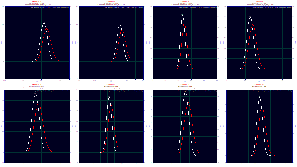
Here we see the opposite of a more conventional fit. The red curve is the unwound GenHVL peak whose deconvolution is the white peak which is actually fitted to the data.
Click on the Numeric button to open the numeric summary and under the Options menu, choose Select Only Fitted Parameters and then check Measured Values, Deconvolved Moments, and Average Multiple Fits. Scroll to the bottom of the report to see the averages.
Average�for�8�Fits
Fitted�Parameters
r2�Coef�Det�� DF�Adj�r2���� Fit�Std�Err�� F-value������ ppm�uVar
0.99999462��� 0.99999427��� 0.07764688��� 11,487,966��� 5.37634646
�Peak�� Type��������� ������a0���� ������a1���� ������a2���� ������a3���� ������a4���� ������a5����
����1�� GenHVL<*g*>�� 6.89666917�� 8.62628210�� 0.02141637�� -2.809e-5��� 0.09235604�� 0.02032334��
Measured�Values
�Peak�� Type��������� �Amplitude�� ��Center���� ���FWHM����� ��Asym50���� �FW�Base���� ��Asym10����
����1�� GenHVL<*g*>�� 152.467810�� 8.61343184�� 0.04407221�� 0.97967742�� 0.08458621�� 0.98022360��
�Peak�� Type��������� ���Area����� ��%�Area���� ���Mean����� ��StdDev���� �Skewness��� �Kurtosis���
����1�� GenHVL<*g*>�� 6.89680489�� 100.000000�� 8.61328246�� 0.01802201�� 0.05505157�� 3.00116728��
CV�Percent�for�8�Fits
Fitted�Parameters
r2�Coef�Det�� DF�Adj�r2���� Fit�Std�Err�� F-value������ ppm�uVar
0.0004103%��� 0.0004413%��� 56.721689%��� 137.08057%��� 76.316998%
�Peak�� Type��������� ������a0���� ������a1���� ������a2���� ������a3���� ������a4���� ������a5����
����1�� GenHVL<*g*>�� 55.781651%�� 8.5812752%�� 5.0519070%�� 22.212627%�� 13.555737%�� 7.8627139%��
Measured�Values
�Peak�� Type��������� �Amplitude�� ��Center���� ���FWHM����� ��Asym50���� �FW�Base���� ��Asym10����
����1�� GenHVL<*g*>�� 59.151496%�� 8.5833565%�� 4.5282845%�� 1.6693250%�� 4.1667426%�� 2.6023313%��
�Peak�� Type��������� ���Area����� ��%�Area���� ���Mean����� ��StdDev���� �Skewness��� �Kurtosis���
����1�� GenHVL<*g*>�� 55.779535%�� 0.0000000%�� 8.5868344%�� 4.3976889%�� 77.946990%�� 1.7087872%
��
While we did not achieve the 2.7 ppm average unaccounted variance, we did realize a 5.4 ppm, appreciably better than the 16.6 ppm of the Gen2HVL direct fits, and the 13.7 ppm of the Gen2HVL<e> attempt to fit the residual IRF. There are two fits below 1 ppm, and the CV% is 76% across the eight fits, with the values ranging from 0.59 ppm to 12.39 ppm.
This type of unwinding estimates the gradient in a5, the deconvolution SD width of the half-Gaussian. The a5 half-Gaussian SD of 0.0204 has a CV% of 7.9%, ranging from 0.0185 to 0.0226. We will need to explore the a5 variable to see if this is related to peak width, the time of exposure to this gradient, or if it may be indicative of the gradient actually having a different strength across time.
We realized this improved accuracy of fit by targeting the actual system model for the gradient. In this case, we used an extremely simple one, a half-Gaussian of SD width .0204 to unwind the gradient compression internally within the model.
We also did this in just one step using the GenHVL<*g*> deconvolution model. In this type of fitting, the sensitivity of goodness of fit to the Fourier domain noise filter is quite high, and as such the filter settings (the S/N threshold) are automatically determined. The filter cannot be manually adjusted.
Click Explore. Only a 2D data visualization is possible. By default x should contain the Data Set number, and y the fitted Parameters.
![]() The Zoom-in Applies to All Graphs will probably be turned on. Click this button in the graph's
toolbar to turn this option off.
The Zoom-in Applies to All Graphs will probably be turned on. Click this button in the graph's
toolbar to turn this option off.
Select Center (a1) for the x variable and Moments for the y variable.
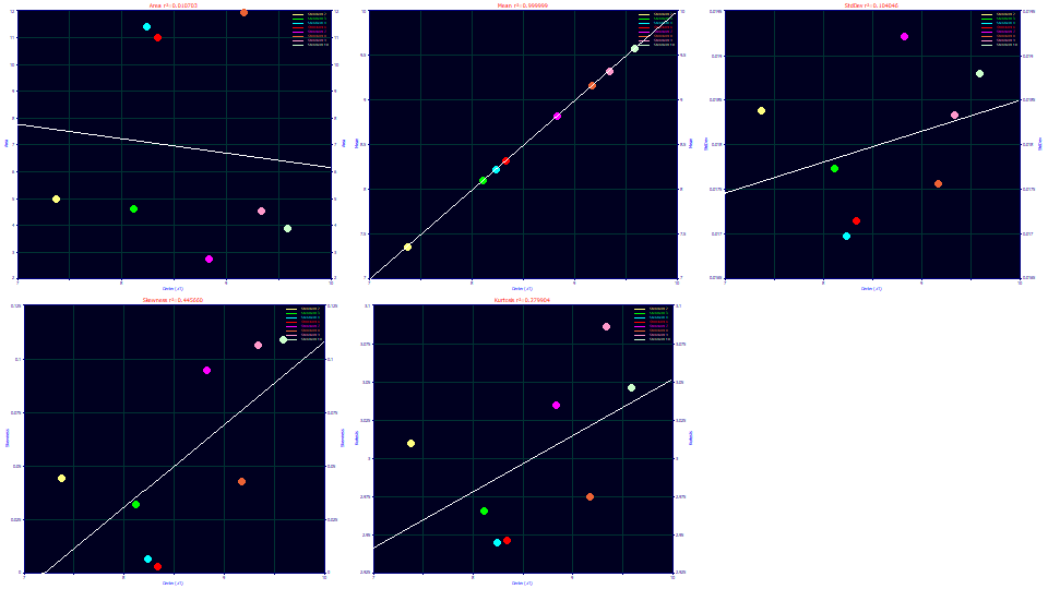
The peaks cannot be assumed to increase in width with increasing elution time. There is a loose correlation where both the skewness and kurtosis increase with elution time. The kurtosis tracks the skewness. This can occur when the the skew produces a fatter tail on right side of the peak while the left side changes little.
Note the scale of the kurtosis, from 2.94 to 3.08. Here we cannot conclude the unwinding was too strong simply because we measure a fourth moment with values below the 3.0 kurtosis of a Gaussian. We know that values less than 3.0 occur on strongly fronted peaks. We will do a final check of the the accuracy of the unwinding by fitting a Gen2HVL<*g*> model. In such a fit we want to see decay powers near 2.0.
Select Width (a2) for the x variable.
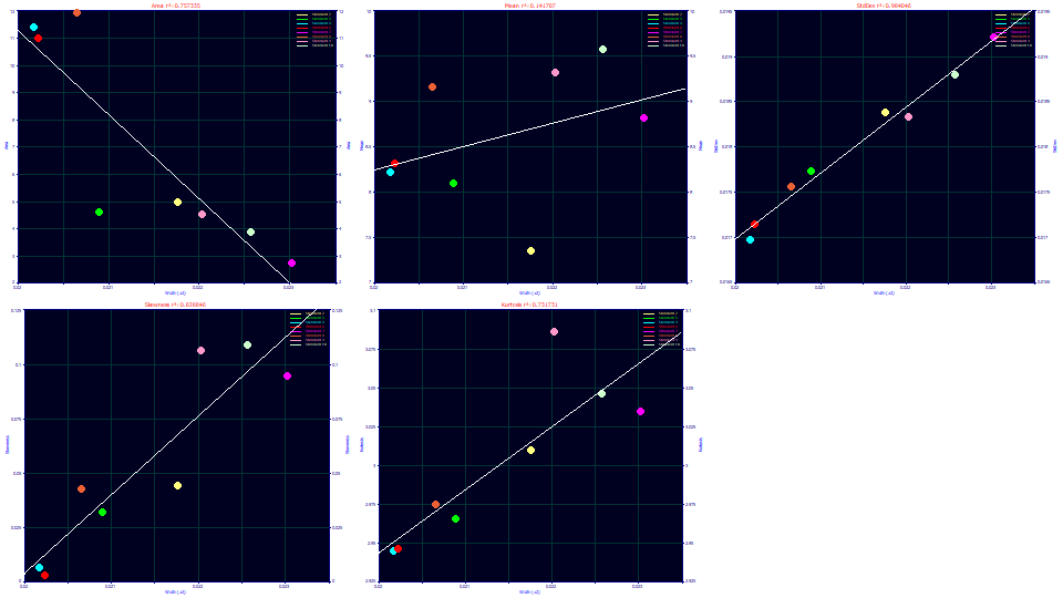
The a2 deconvolved Gaussian width strongly tracks the second moment as expected. Here there is a very good correlation between width and the skewness, and again the right tailing arising from the skew directly impacts the fourth moment.
Select Distortion (a3) for the x variable.
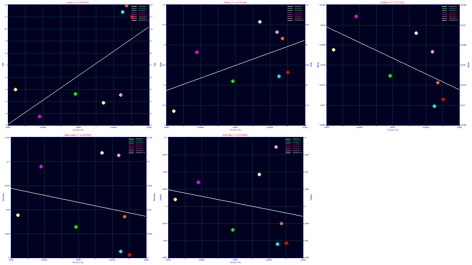
The a3 chromatographic distortion roughly increases with the a1 retention time, which is what might be expected with an isocratic separation (going from a negative fronting to a positive tailing with elution time). There is also a rough inverse correlation with the second moment (as an SD).
Select Parameter (a4) for the x variable.
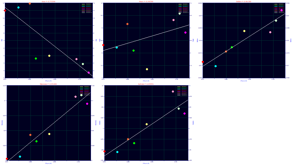
The a4 term is the ZDD asymmetry, and it is clearly strongly correlated with the peak skewness, and again the kurtosis tracks the tailing arising from the skew. There is also a strong relationship between the SD of the peak and the ZDD asymmetry.
Select Parameter (a5) for the x variable.
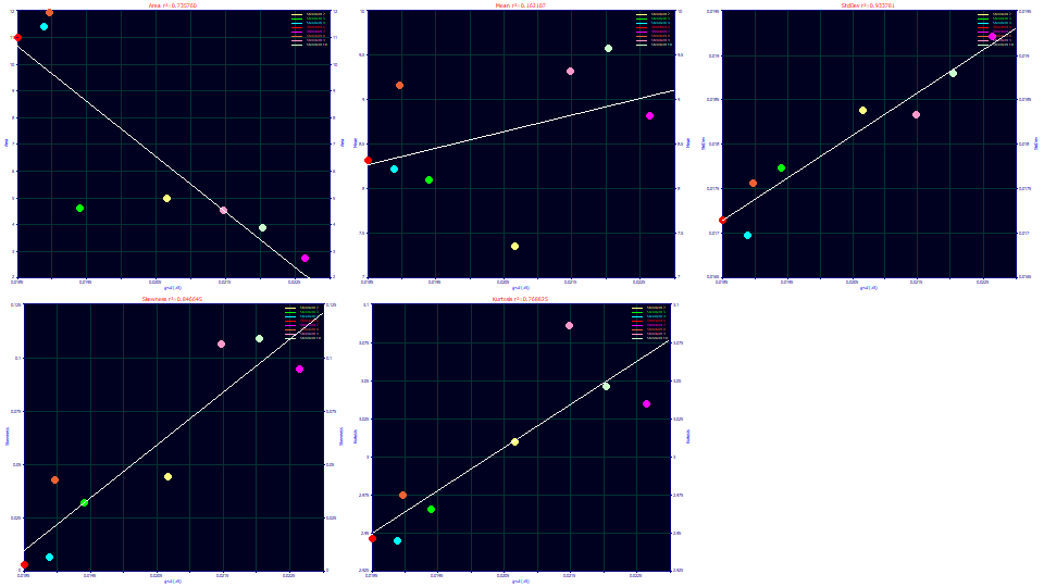
The a5 parameter is is the width of the half-Gaussian performing the unwinding. The greater the width of the peak, the greater the measure of unwinding required, and the correlation is a strong one. The peaks are not constant in width; they vary somewhat from .017 to .019 in the second moment SD. The measure of half-Gaussian unwinding appears to be proportional to the width. Once again we see that the skew and kurtosis track one another as they track the SD, something that would not happen if the unwinding was unsuccessful.
Although the unwinding was imperfect, we can conclude the unwound peaks adopt a skew with additional exposure to the gradient and that the unwinding is not equal because the gradient is not equal in its influence upon the different solutes. Peaks that see a greater time of exposure to the gradient, which have a higher second moment SD, are more right skewed.
Click OK to close the Explore dialog, OK to close the Review, OK to accept a saved GenHVL<*g*> fit in the data file, OK to acknowledge the revision in the file. Remain in the placement screen.
Confirming the Unwinding of the Gradient with the Gen2HVL<*g*> Deconvolution Model
The Gen2HVL<*g*> model is identical to the GenHVL<*g*> except that a power of decay, a fourth moment term adjustment, is also fitted. If the gradient has been successfully unwound, and assuming global maximum fits are realized with better goodness of fits than the GenHVL<*g*> model (the twice generalized model is more prone to local minima in the fitting process), the power of decay parameter should be very close to 2.0, the expected isocratic value.
From the Chromatography w/IRF family, change the model to the Gen2HVL<*g*>.
Click Peak Fit to open the fit strategy dialog. Select the Fit with Reduced Data Prefit, 2 Pass, Lock Shared Parameters on Pass 1. Leave the Fit using Sequential Constraints box checked. Click OK. Again we use the two-pass option to hold the higher moment parameters constant while the main peak parameters are first estimated, and only thereafter are the a4 and a5 ZDD and a6 IRF parameters fitted. This is especially important when both higher moments are fitted in the ZDD zero distortion density.
Click Review Fit.
![]() Once again,click the Hide
Y2 plot in the graph's toolbar.
Once again,click the Hide
Y2 plot in the graph's toolbar.
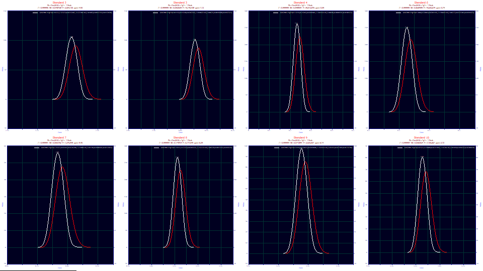
Click on the Numeric button to open the numeric summary. Scroll to the bottom of the report to see the averages.
Average�for�8�Fits
Fitted�Parameters
r2�Coef�Det�� DF�Adj�r2���� Fit�Std�Err�� F-value������ ppm�uVar
0.99999600��� 0.99999569��� 0.06955302��� 11,358,231��� 3.99771183
�Peak�� Type��������� ������a0���� ������a1���� ������a2���� ������a3���� ������a4���� ������a5���� ������a6����
����1�� Gen2HVL<*g*>�� 6.89623880�� 8.62553372�� 0.02112483�� -2.623e-5��� 2.01025225�� 0.08422079�� 0.01918017��
Measured�Values
�Peak�� Type���������� �Amplitude�� ��Center���� ���FWHM����� ��Asym50���� �FW�Base���� ��Asym10����
����1�� Gen2HVL<*g*>�� 152.444880�� 8.61336574�� 0.04407971�� 0.98629862�� 0.08459111�� 0.98318758��
�Peak�� Type���������� ���Area����� ��%�Area���� ���Mean����� ��StdDev���� �Skewness��� �Kurtosis���
����1�� Gen2HVL<*g*>�� 6.89634909�� 100.000000�� 8.61314384�� 0.01800067�� 0.06155052�� 2.95935921��
CV�Percent�for�8�Fits
Fitted�Parameters
r2�Coef�Det�� DF�Adj�r2���� Fit�Std�Err�� F-value������ ppm�uVar
0.0003219%��� 0.0003497%��� 65.278094%��� 115.98030%��� 80.539347%
�Peak�� Type��������� ������a0���� ������a1���� ������a2���� ������a3���� ������a4���� ������a5���� ������a6����
����1�� Gen2HVL<*g*>�� 55.788764%�� 8.5768028%�� 4.4263235%�� 21.730965%�� 0.5317225%�� 10.723590%�� 6.6844590%��
Measured�Values
�Peak�� Type���������� �Amplitude�� ��Center���� ���FWHM����� ��Asym50���� �FW�Base���� ��Asym10����
����1�� Gen2HVL<*g*>�� 59.161113%�� 8.5833617%�� 4.5294653%�� 1.8647009%�� 4.1683970%�� 2.6999618%��
�Peak�� Type���������� ���Area����� ��%�Area���� ���Mean����� ��StdDev���� �Skewness��� �Kurtosis���
����1�� Gen2HVL<*g*>�� 55.786817%�� 0.0000000%�� 8.5857264%�� 4.3273699%�� 110.35306%�� 0.5747950%��
The average 3.99 ppm error is better then the GenHVL<*g*>, but that would be expected. Here we see an average power of decay of 2.01 across the eight fits, with a CV% of 0.53, ranging from 2.000 to 2.0344. With the estimates of the power, the half-Gaussian width dropped slightly from .0203 to .0192. We can conclude the unwinding in the data was generally good. We have at least an approximation to the isocratic peaks.
Click Explore. Select Parameter (a4) for the x variable and Moments for the y variable.
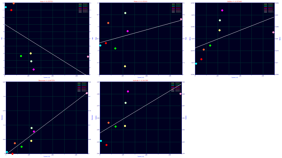
Note that one of the eight fits is an outlier with respect to the other seven. With this one exception, all are very close to 2.0 in the a4 decay power.
Click OK to close the Explore dialog, OK to close the Review, OK to accept a saved Gen2HVL<*g*> fit in the data file, and OK to acknowledge the revision in the file. Remain in the placement screen.
Fitting the Gradient using the GenHVL<*k*> Deconvolution Model
From the Chromatography w/IRF family, change the model to the GenHVL<*k*>. This is the only other built-in IRF model we have found to unwind an HPLC gradient successfully. It is a two-parameter variable order kinetic IRF. When the order is 0, there is a simple linear decay, and when the order is 1, there is an exponential decay. Our experience is such we expect to see an order of decay that is about 0.7, between the two.
Here you will see the 'k' IRF defaults are strong (too much deconvolution is occurring).
Click the IRF button and for the <k> IRF, enter 0.7 for the k order default starting estimate, and 0.15 for the k width tau. Click OK.
Click Peak Fit to open the fit strategy dialog. Select the Fit with Reduced Data Prefit, 2 Pass, Lock Shared Parameters on Pass 1. Leave the Fit using Sequential Constraints box checked. Click OK. Again we use the two-pass option to hold the higher moment parameters constant while the main peak parameters are first estimated, and only thereafter are the a4 ZDD and the a5 and a6 IRF parameters fitted. This is especially important with two parameter IRFs.
Click Review Fit.
![]() Once again,click the Hide
Y2 plot in the graph's toolbar.
Once again,click the Hide
Y2 plot in the graph's toolbar.
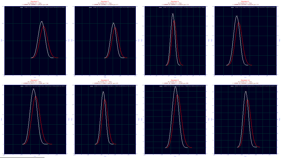
Click on the Numeric button to open the numeric summary. Scroll to the bottom of the report to see the averages.
Average�for�8�Fits
Fitted�Parameters
r2�Coef�Det�� DF�Adj�r2���� Fit�Std�Err�� F-value������ ppm�uVar
0.99999430��� 0.99999386��� 0.08143477��� 5,759,968���� 5.70408348
�Peak�� Type��������� ������a0���� ������a1���� ������a2���� ������a3���� ������a4���� ������a5���� ������a6����
����1�� GenHVL<*k*>�� 6.89732953�� 8.62310476�� 0.02081013�� -3.058e-5��� 0.09492934�� 0.02122031�� 0.71311845��
Measured�Values
�Peak�� Type��������� �Amplitude�� ��Center���� ���FWHM����� ��Asym50���� �FW�Base���� ��Asym10����
����1�� GenHVL<*k*>�� 152.508751�� 8.61345931�� 0.04405756�� 0.97642764�� 0.08461173�� 0.98006855��
�Peak�� Type��������� ���Area����� ��%�Area���� ���Mean����� ��StdDev���� �Skewness��� �Kurtosis���
����1�� GenHVL<*k*>�� 6.89745176�� 100.000000�� 8.61325485�� 0.01801855�� 0.07101287�� 3.02129202��
CV�Percent�for�8�Fits
Fitted�Parameters
r2�Coef�Det�� DF�Adj�r2���� Fit�Std�Err�� F-value������ ppm�uVar
0.0003714%��� 0.0004033%��� 31.344938%��� 114.86384%��� 65.121573%
�Peak�� Type��������� ������a0���� ������a1���� ������a2���� ������a3���� ������a4���� ������a5���� ������a6����
����1�� GenHVL<*k*>�� 55.822939%�� 8.5867423%�� 4.2954522%�� 25.623660%�� 13.978366%�� 11.617192%�� 8.6264160%��
Measured�Values
�Peak�� Type��������� �Amplitude�� ��Center���� ���FWHM����� ��Asym50���� �FW�Base���� ��Asym10����
����1�� GenHVL<*k*>�� 59.154430%�� 8.5831838%�� 4.5290707%�� 1.7044062%�� 4.1804780%�� 2.6125143%��
�Peak�� Type��������� ���Area����� ��%�Area���� ���Mean����� ��StdDev���� �Skewness��� �Kurtosis���
����1�� GenHVL<*k*>�� 55.820750%�� 0.0000000%�� 8.5878134%�� 4.2077828%�� 61.069305%�� 3.3224849%��
The average 5.70 ppm error is higher than the single parameter half-Gaussian IRF average of 5.38 for the eight fits. The CV% on the goodness of fit is 65%, better than the half-Gaussian, the values ranging from 1.10 ppm to 11.62 ppm.
It should be noted that kinetic powers between .55 and .75 can strongly approximate half-Gaussian decays, or conversely, half-Gaussian decays can very effectively approximate kinetic decays of .55 to .75 fractional order. Despite the apparent differences, the distortion being deconvolved is quite similar between the two models.
Click OK to close the Review, OK to accept a saved GenHVL<*k*> fit in the data file, OK to acknowledge the revision in the file, and OK tor return to the placement window.
Confirming the Unwinding of the Gradient with the Gen2HVL<*k*> Deconvolution Model
We will do one more fit with the Gen2HVL<*k*> model to confirm the unwinding in the GenHVL<*k*> model.
From the Chromatography w/IRF family, change the model to the Gen2HVL<*k*>.
Click Peak Fit to open the fit strategy dialog. Select the Fit with Reduced Data Prefit, 2 Pass, Lock Shared Parameters on Pass 1. Leave the Fit using Sequential Constraints box checked. Click OK.
Click Review Fit. If needed, click on the Numeric button to open the numeric summary. Scroll to the bottom of the report to see the averages.
Average�for�8�Fits
Fitted�Parameters
r2�Coef�Det�� DF�Adj�r2���� Fit�Std�Err�� F-value������ ppm�uVar
0.99999719��� 0.99999694��� 0.05769172��� 11,476,787��� 2.81402332
�Peak�� Type��������� ������a0���� ������a1���� ������a2���� ������a3���� ������a4���� ������a5���� ������a6�������������a7������������
����1�� Gen2HVL<*k*>�� 6.89692315�� 8.62261064�� 0.02055266�� -2.585e-5��� 2.02000300�� 0.08010792�� 0.01994034�� 0.70132665��
Measured�Values
�Peak�� Type���������� �Amplitude�� ��Center���� ���FWHM����� ��Asym50���� �FW�Base���� ��Asym10����
����1�� Gen2HVL<*k*>�� 152.403597�� 8.61333934�� 0.04407323�� 0.98790980�� 0.08462838�� 0.98546369��
�Peak�� Type���������� ���Area����� ��%�Area���� ���Mean����� ��StdDev���� �Skewness��� �Kurtosis���
����1�� Gen2HVL<*k*>�� 6.89705367�� 100.000000�� 8.61326473�� 0.01799804�� 0.04116050�� 2.96583651��
CV�Percent�for�8�Fits
Fitted�Parameters
r2�Coef�Det�� DF�Adj�r2���� Fit�Std�Err�� F-value������ ppm�uVar
0.0002200%��� 0.0002411%��� 47.597992%��� 125.18888%��� 78.200842%
�Peak�� Type��������� ������a0���� ������a1���� ������a2���� ������a3���� ������a4���� ������a5���� ������a6�������������a7������������
����1�� Gen2HVL<*k*>�� 55.820619%�� 8.5848132%�� 4.1142494%�� 26.229531%�� 0.8165838%�� 13.359164%�� 13.629707%�� 9.4698904%��
Measured�Values
�Peak�� Type���������� �Amplitude�� ��Center���� ���FWHM����� ��Asym50���� �FW�Base���� ��Asym10����
����1�� Gen2HVL<*k*>�� 59.180802%�� 8.5830160%�� 4.5316754%�� 2.0313119%�� 4.1907114%�� 2.7873510%��
�Peak�� Type���������� ���Area����� ��%�Area���� ���Mean����� ��StdDev���� �Skewness��� �Kurtosis���
����1�� Gen2HVL<*k*>�� 55.818540%�� 0.0000000%�� 8.5868108%�� 4.1718965%�� 82.454341%�� 1.4427246%��
The average 2.81 ppm error is better then the 4.0 of the Gen2HVL<*g*>. When the power of decay is accounted, the extra parameter in the <*k*> deconvolution did produce a benefit. Here we see an average power of decay of 2.02 across the eight fits, with a CV% of 0.81, weaker than the Gen2HVL<*g*>. With the estimates of the power, the variable order kinetic response function power dropped slightly from 0.713 to 0.701, and the k time constant dropped from 0.02122 to 0.0199.
Here as well we can conclude the unwinding in the data was generally good and that we have a fair a fair approximation to the isocratic peaks.
Click OK to close the Review, OK to accept a saved Gen2HVL<*k*> fit in the data file, OK to acknowledge the revision in the file, OK to return to the placement screen, and OK one final time to return to main window.
Differences between Fits of Compressed vs. Unwound Gradient Data
We will now compare the average of the Gen2HVL direct fits in the first gradient peaks tutorial with the averages of the eight fits we just made:
|
Model |
a0 |
a1 |
a2 |
a3 |
a4 |
a5 |
a6 |
a7 |
F-stat |
ppm�uVar |
|
Gen2HVL |
6.89712 |
8.61235 |
0.01836 |
-6.535E-06 |
2.13182 |
0.00782 |
|
|
1,259,491 |
16.66 |
|
GenHVL<*g*> |
6.89667 |
8.62628 |
0.02142 |
-2.809E-05 |
0.09236 |
0.02032 |
|
|
11,487,966 |
5.38 |
|
Gen2HVL<*g*> |
6.89624 |
8.62553 |
0.02112 |
-2.623E-05 |
2.01025 |
0.08422 |
0.01918 |
|
11,358,231 |
4.00 |
|
GenHVL<*k*> |
6.89733 |
8.62310 |
0.02081 |
-3.058E-05 |
0.09493 |
0.02122 |
0.71312 |
|
5,759,968 |
5.70 |
|
Gen2HVL<*k*> |
6.89692 |
8.62261 |
0.02055 |
-2.585E-05 |
2.02000 |
0.08011 |
0.01994 |
0.70132 |
11,476,787 |
2.81 |
The a0 area is unimpacted.
The a1 deconvolved Gaussian mean shifts slightly upward with the unwinding.
The a2 deconvolved Gaussian SD is higher than the direct fit of the compressed shape, reflecting the unwinding of the gradient.
The a3 chromatographic distortion in the internal unwinding is about 5x higher in magnitude than the value seen with the direct compressed fit.
The ZDD asymmetry fit to 0.0078 without the unwinding, and to 0.080-0.094 after the unwinding, about 10-12x higher.
The Power of Decay fit to 2.13 without the unwinding, and to 2.01-2.02 after the unwinding. A 2.0 power with low scatter would represent an optimal unwinding.
The IRF 'g' SD and 'k' time constant both fit to a narrow 0.0191-0.0212 range.
The IRF 'k' power of decay fit to 0.701-0.713.
In the first gradient tutorial we looked at the different closed form direct fits of the gradient shapes and struggled to find differences in the average F-statistic. That is not an issue here as the average F-statistic increases to 11.5 million. Because the GenHVL<*g*> accomplishes with one parameter that which the GenHVL<*k*> realizes only with two, the F-statistic is much higher for the GenHVL<*g*> model and from an information theoretic perspective is the better model to describe the data.
As we noted above, the core chromatographic parameters are impacted by the unwinding. Even the a1 location will shift slightly. Only the a0 area is unimpacted since the deconvolution is area invariant. When you are fitting a direct closed form model, you are estimating the gradient with the fourth moment and the compressed shape is fitted as if it were an isocratic elution. When you fit a deconvolution model, you estimate the gradient with a deconvolution IRF, and you fit an uncompressed (unwound) shape.
The Estimated Constant Mobile Phase Peaks
In the Saved Fits dropdown, select the GenHVL<*g*> fit. This will reopen the Review with this specific fit. Be sure As Fitted is in the first dropdown, IRF Deconv. is in the second, Partial Deconv. is in the third, and Full Deconv. is in the fourth. Double click the third graph, the fit with the .59 ppm.
![]() Once again,click the Hide Y2 plot in the graph's toolbar. Zoom-in the peaks.
Once again,click the Hide Y2 plot in the graph's toolbar. Zoom-in the peaks.
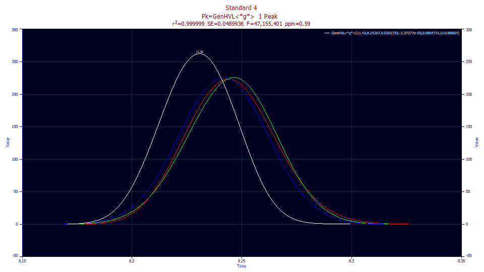
In this case, the peaks minus the IRF (gradient) look very different. The red curve is the GenHVL peak which is estimated to exist were no gradient present. The green peak, with its fronted shape, is the pure HVL with the ZDD distortions removed. The blue peak is the pure Gaussian with all distortions removed, including the a3 concentration-dependent chromatographic distortion. The green HVL is thus the pure chromatographic peak one would expect to see in a constant mobile phase elution. The blue Gaussian is the peak estimated to exist with no gradient, no ZDD non-ideality, and no concentration-dependent a3 distortion (the peak that would be observed as the concentration approaches an infinite dilution).
The different direction arising from fitting a deconvolution model as the IRF, rather than a convolution, does require some acclimation. All of the estimated constant mobile phase 'deconvolutions' are broadened rather than sharpened because the IRF is a deconvolution (narrowing) instead of a convolution (widening). You are still looking at deconvolutions, as in the green peak removing the smearing from the ZDD non-ideality, and the blue peak further removing the intrinsic a3 chromatographic distortion. The adjustment rests in appreciating that the IRF deconvolution is the removal of the gradient, a process that broadens rather than sharpens the resultant shape.
Note that fitting a conventional IRF using a convolution integral requires baseline-resolved peaks where the introduced tails from the IRF are visible and can be fitted. The same issue exists in a deconvolution model since the gradient's strongest presence will rest in the thinning of the tails of the peaks. You will need to accurately fit this fourth moment thinning if the deconvolution fits are to successfully recover estimates of what the peaks would look like in a constant mobile phase elution, and if the gradient itself is to be accurately estimated.
Click OK to close the Review.
In thus tutorial, we fit the gradient as an IRF in a single step fitting which deconvolved the pure chromatographic peaks. In the third of the gradient peak tutorials, we will explore the two step process of fitting unwound data.