PeakLab v1 Documentation Contents AIST Software Home AIST Software Support
IRF Estimation 3 - Standards Containing Only Tailed Peaks
In this final approach to estimating an IRF , we will estimate the IRF using only tailed peaks.
In the IRF Estimation 2 topic, the difficulty of estimating tailed peaks was discussed. Estimating the IRF from only intrinsically tailed peaks is a worst-case scenario. In estimating an IRF it is best if the a3 intrinsic chromatographic distortion is fronted, in the opposite direction of the IRF, which will be tailed. In other words, we would like one or more a negative a3 (intrinsically fronted) peaks to be used for the IRF determination.
If you must estimate the IRF from tailed peaks, such is possible, but it will require some additional effort. Because of the correlation between the instrumental tailing and the intrinsic chromatographic tailing, you will have to help the fitting process along. This can be straightforward. If you fit GenHVL or GenNLC peaks, you will generally have a good estimate of the deviation from non-ideality for the ZDD zero-distortion density. The program's default for the GenNLC in the ZDD dialog is 1.1858. The pure HVL is 0 and the pure NLC is 0.5. If your experience parallels ours, you will have a infinite dilution density with a skewness that is in the vicinity of 2-3x that of the Giddings density (which produces the NLC). Also, if you fit <ge> IRFs, you will rather quickly come to know the area fraction of your narrow and wide components. In the IRF dialog, our default for the <ge> is a g area fraction of 0.6113 (this is for the narrow component). We generally see about 5/8 of the overall IRF area attributable to the narrow width component, and about 3/8 area to the wider exponential. If we lock these two values in a fit, we can often stop much of this intercorrelation between the two different types of tailing.
Tailed Peak IRF Estimation
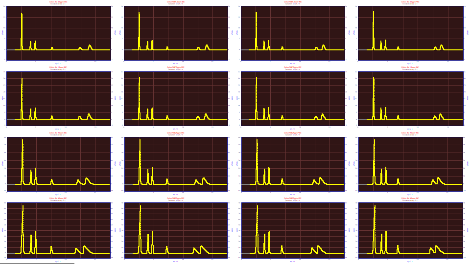
For this example, we will use this same six-peak cation standard, and we will isolate and fit the three tailed peaks in order to estimate the IRF. Here we will use a matrix of concentration (5-10-25-50 ppm) and temperature (30-35-40-45C) as the data we will average for the estimate. We use this data instead of the data in the fronted examples, since the additive impacted the IRF, and we know the tailed peak IRF estimation is going to be more challenging. Since this is different data, we will first do a full fit with the fronted peaks to establish an expectation for the tailed IRF estimation.

If we fit these 16 data sets to the GenHVL<ge> with the a4 ZDD asymmetry and a5-a6 IRF parameters shared across all peaks, and the IRF narrow width a7 fraction locked at 0.625, we see the following when these 16 sets are averaged using the Average Multiple Fits option in the Numeric Summary.
AverageĀforĀ16ĀFits
FittedĀParameters
r2 ĀCoefĀDetĀĀ DFĀAdjĀr 2ĀĀĀĀ FitĀStdĀErr ĀĀ F-value ĀĀĀĀĀĀ ppmĀuVar
0.99998921ĀĀĀ 0.99998918 ĀĀĀ 0.01629336 ĀĀĀ 50,476,703 ĀĀĀ 10.7917053
ĀPeakĀĀ TypeĀĀĀĀĀĀĀĀ ĀĀĀĀĀĀa0ĀĀ ĀĀ ĀĀĀĀĀĀa1ĀĀ ĀĀ ĀĀĀĀĀĀa2ĀĀ ĀĀ ĀĀĀĀĀĀa3ĀĀ ĀĀ ĀĀĀĀĀĀa4ĀĀ ĀĀ ĀĀĀĀĀĀa5ĀĀ ĀĀ ĀĀĀĀĀĀa6ĀĀ ĀĀ ĀĀĀĀĀĀa7ĀĀ ĀĀ
ĀĀĀĀ1ĀĀ GenNLC<ge> ĀĀ 8.26155931 ĀĀ 2.44289465 ĀĀ 0.00024648 ĀĀ -0.0101086 ĀĀ 1.20820068 ĀĀ 0.00810942 ĀĀ 0.04431287 ĀĀ 0.62500000 ĀĀ
ĀĀĀĀ2ĀĀ GenNLC<ge> ĀĀ 2.32025938 ĀĀ 3.85936993 ĀĀ 0.00027942 ĀĀ -0.0018371 ĀĀ 1.20820068 ĀĀ 0.00810942 ĀĀ 0.04431287 ĀĀ 0.62500000 ĀĀ
ĀĀĀĀ3ĀĀ GenNLC<ge> ĀĀ 2.69783874 ĀĀ 4.64491174 ĀĀ 0.00027237 ĀĀ -0.0011021 ĀĀ 1.20820068 ĀĀ 0.00810942 ĀĀ 0.04431287 ĀĀ 0.62500000 ĀĀ
ĀĀĀĀ4ĀĀ GenNLC<ge> ĀĀ 1.21948046 ĀĀ 7.11781529 ĀĀ 0.00037808 ĀĀ 0.00162510 ĀĀ 1.20820068 ĀĀ 0.00810942 ĀĀ 0.04431287 ĀĀ 0.62500000 ĀĀ
ĀĀĀĀ5ĀĀ GenNLC<ge> ĀĀ 2.07696389 ĀĀ 12.6150205 ĀĀ 0.00076793 ĀĀ 0.01235987 ĀĀ 1.20820068 ĀĀ 0.00810942 ĀĀ 0.04431287 ĀĀ 0.62500000 ĀĀ
ĀĀĀĀ6ĀĀ GenNLC<ge> ĀĀ 4.21397004 ĀĀ 14.1049378 ĀĀ 0.00088484 ĀĀ 0.02803543 ĀĀ 1.20820068 ĀĀ 0.00810942 ĀĀ 0.04431287 ĀĀ 0.62500000 ĀĀ
With the 0.0081 narrow width half-Gaussian SD and the 0.0443 exponential time constant we have confirmed the two key IRF widths from the IRF Estimation 1 and IRF Estimation 2 examples. We also see the a4 ZDD asymmetry of 1.2082 very close to the program's default of 1.1858. We will need the a4 of 1.2082 and the a7 of 0.625 for this tailed peak estimation fitting.
It is sometimes instructive to use the above fit as a starting point to see if the a5 and a6 narrow and wide component of the IRF are changing in any discernible trend. We use the right click Set Common Parameters Across Peaks For All Data Sets... menu option to lock the a4 ZDD asymmetry at 1.2082 for all fits, to lock the a7 narrow component fraction of the IRF at .625 of the area, and we open up a5 and a6 to vary on a per peak basis:
AverageĀforĀ16ĀFits
FittedĀParameters
r2ĀCoefĀDet ĀĀ DFĀAdjĀr2 ĀĀĀĀ FitĀStdĀErrĀĀ F-value ĀĀĀĀĀĀ ppmĀuVar
0.99999123ĀĀĀ 0.99999120ĀĀĀ 0.01480487ĀĀĀ 45,916,924 ĀĀĀ 8.77443472
ĀPeakĀĀ TypeĀĀĀĀĀĀĀĀ ĀĀĀĀĀĀa0ĀĀĀĀ ĀĀĀĀĀĀa1ĀĀĀĀ ĀĀĀĀĀĀa2ĀĀĀĀ ĀĀĀĀĀĀa3ĀĀ ĀĀ ĀĀĀĀĀĀa4ĀĀĀĀ ĀĀĀĀĀĀa5ĀĀ ĀĀ ĀĀĀĀĀĀa6ĀĀĀĀ ĀĀĀĀĀĀa7ĀĀ ĀĀ
ĀĀĀĀ1ĀĀ GenNLC<ge>ĀĀ 8.26338310ĀĀ 2.44283955 ĀĀ 0.00024469ĀĀ -0.0100655 ĀĀ 1.20820000ĀĀ 0.00819214 ĀĀ 0.04446035ĀĀ 0.62500000 ĀĀ
ĀĀĀĀ2ĀĀ GenNLC<ge>ĀĀ 2.31925724ĀĀ 3.86032380 ĀĀ 0.00027733ĀĀ -0.0018581 ĀĀ 1.20820000ĀĀ 0.00547038 ĀĀ 0.04391348ĀĀ 0.62500000 ĀĀ
ĀĀĀĀ3ĀĀ GenNLC<ge>ĀĀ 2.69220169ĀĀ 4.64808833 ĀĀ 0.00027252ĀĀ -0.0011007 ĀĀ 1.20820000ĀĀ 0.00328424 ĀĀ 0.04173921ĀĀ 0.62500000 ĀĀ
ĀĀĀĀ4ĀĀ GenNLC<ge>ĀĀ 1.22244426ĀĀ 7.11373675 ĀĀ 0.00037659ĀĀ 0.00158623 ĀĀ 1.20820000ĀĀ 0.01251984 ĀĀ 0.04685827ĀĀ 0.62500000 ĀĀ
ĀĀĀĀ5ĀĀ GenNLC<ge>ĀĀ 2.07569340ĀĀ 12.6206726 ĀĀ 0.00077245ĀĀ 0.01237467 ĀĀ 1.20820000ĀĀ 0.01113443 ĀĀ 0.02724279ĀĀ 0.62500000 ĀĀ
ĀĀĀĀ6ĀĀ GenNLC<ge>ĀĀ 4.21586319ĀĀ 14.1099190 ĀĀ 0.00090909ĀĀ 0.02822314 ĀĀ 1.20820000ĀĀ 0.00863092 ĀĀ 0.02925939ĀĀ 0.62500000 ĀĀ
Ā
With respect to the a6 exponential component, the one we expect to be close to constant, peak 4, potassium, which is only modestly tailed, is in reasonably good agreement with the three fronted peaks. The much later eluting calcium and magnesium, peaks 5 and 6, are extremely tailed, and their averages are not in agreement with the the first four peaks.
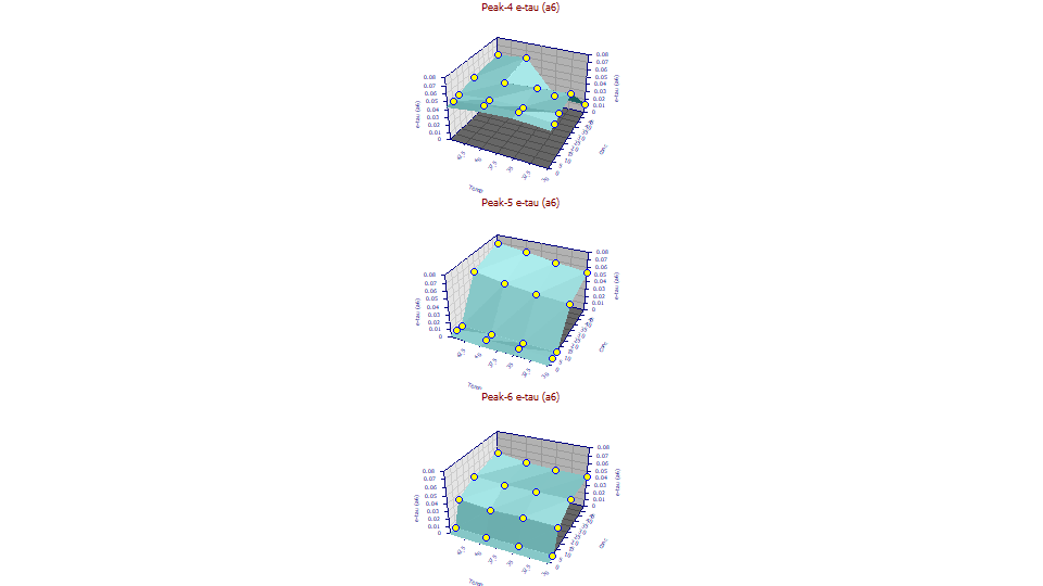
If we use the Explore option to look at the Conc vs Temp surfaces for the a6 exponential width in the IRF, only the slightly tailed fourth peak has a6 reasonably constant at most temperatures and concentrations. All is good at the 5,10,25 ppm concentration, but at the 30C and 35C temperatures and 50ppm, the a6 value falls off a cliff. For peaks 5 and 6, there is no constancy. We think it is due to the Ca+ and Mg+ interacting differently at different concentrations. If we average peak 5 or peak 6, we would have to limit the average to the 25 and 50 ppm concentrations. If we do this:
PeakĀ4:ĀPotassium
AverageĀforĀ14ĀFits
FittedĀParameters
r2ĀĀCoefĀDetĀ DFĀAdjĀr2ĀĀ FitĀStdĀErrĀ F-valueĀ ppmĀuVar
0.99999232Ā 0.99999230Ā 0.01160998Ā 49,648,269Ā 7.67759619
ĀPeakĀ TypeĀĀĀĀĀĀĀĀ ĀĀĀa0ĀĀĀĀĀĀ ĀĀĀa1ĀĀĀĀĀĀĀ ĀĀĀa2ĀĀĀĀĀĀ ĀĀĀĀa3ĀĀĀĀĀĀ ĀĀĀĀa4ĀĀĀĀĀ ĀĀĀa5ĀĀĀĀĀĀĀ ĀĀĀĀa6ĀĀĀĀĀ ĀĀĀĀa7ĀĀĀĀĀ
ĀĀĀĀ1Ā GenNLC<ge>ĀĀ 6.80469758Ā 2.45061807ĀĀ 0.00023824Ā -0.0083379ĀĀ 1.20820000Ā 0.00809840ĀĀ 0.04451166Ā 0.62500000Ā
ĀĀĀĀ2Ā GenNLC<ge>ĀĀ 1.91015205Ā 3.85383405ĀĀ 0.00027029Ā -0.0015466ĀĀ 1.20820000Ā 0.00474402ĀĀ 0.04398425Ā 0.62500000Ā
ĀĀĀĀ3Ā GenNLC<ge>ĀĀ 2.21744955Ā 4.63842330ĀĀ 0.00026814Ā -0.0009203ĀĀ 1.20820000Ā 0.00253383ĀĀ 0.04178367Ā 0.62500000Ā
ĀĀĀĀ4Ā GenNLC<ge>ĀĀ 1.00811714Ā 7.06415436ĀĀ 0.00036583Ā 0.00113263ĀĀ 1.20820000Ā 0.01314113ĀĀ 0.05167537Ā 0.62500000Ā
ĀĀĀĀ5Ā GenNLC<ge>ĀĀ 1.71319123Ā 12.6583478ĀĀ 0.00077102Ā 0.01025733ĀĀ 1.20820000Ā 0.00940577ĀĀ 0.02328284Ā 0.62500000Ā
ĀĀĀĀ6Ā GenNLC<ge>ĀĀ 3.47344205Ā 14.1039501ĀĀ 0.00089252Ā 0.02321374ĀĀ 1.20820000Ā 0.00830972ĀĀ 0.02742569Ā 0.62500000
Peak 5: Calcium, Peak 6: Magnesium
AverageĀforĀ8ĀFits
FittedĀParameters
r2ĀCoefĀDetĀĀ DFĀAdjĀr2ĀĀĀĀ FitĀStdĀErrĀĀ F-valueĀĀĀĀĀĀ ppmĀuVar
0.99998861ĀĀĀ 0.99998857ĀĀĀ 0.02513012ĀĀĀ 38,864,837ĀĀĀ 11.3910230
ĀPeakĀĀ TypeĀĀĀĀĀĀĀĀ ĀĀĀĀĀĀa0ĀĀĀĀ ĀĀĀĀĀĀa1ĀĀĀĀ ĀĀĀĀĀĀa2ĀĀĀĀ ĀĀĀĀĀĀa3ĀĀĀĀ ĀĀĀĀĀĀa4ĀĀĀĀ ĀĀĀĀĀĀa5ĀĀĀĀ ĀĀĀĀĀĀa6ĀĀĀĀ ĀĀĀĀĀĀa7ĀĀĀĀ
ĀĀĀĀ1ĀĀ GenNLC<ge>ĀĀ 13.7794738ĀĀ 2.41414124ĀĀ 0.00026231ĀĀ -0.0166604ĀĀ 1.20820000ĀĀ 0.00917166ĀĀ 0.04430576ĀĀ 0.62500000ĀĀ
ĀĀĀĀ2ĀĀ GenNLC<ge>ĀĀ 3.86755142ĀĀ 3.84323169ĀĀ 0.00029493ĀĀ -0.0031048ĀĀ 1.20820000ĀĀ 0.00968468ĀĀ 0.04385163ĀĀ 0.62500000ĀĀ
ĀĀĀĀ3ĀĀ GenNLC<ge>ĀĀ 4.49040808ĀĀ 4.63614358ĀĀ 0.00028285ĀĀ -0.0018829ĀĀ 1.20820000ĀĀ 0.00576324ĀĀ 0.04120821ĀĀ 0.62500000ĀĀ
ĀĀĀĀ4ĀĀ GenNLC<ge>ĀĀ 2.03869859ĀĀ 7.11493858ĀĀ 0.00038184ĀĀ 0.00278443ĀĀ 1.20820000ĀĀ 0.01568341ĀĀ 0.04447756ĀĀ 0.62500000ĀĀ
ĀĀĀĀ5ĀĀ GenNLC<ge>ĀĀ 3.46263262ĀĀ 12.5467763ĀĀ 0.00072954ĀĀ 0.02020473ĀĀ 1.20820000ĀĀ 0.02115366ĀĀ 0.05390487ĀĀ 0.62500000ĀĀ
ĀĀĀĀ6ĀĀ GenNLC<ge>ĀĀ 7.02979774ĀĀ 14.1154960ĀĀ 0.00093248ĀĀ 0.04690095ĀĀ 1.20820000ĀĀ 0.01267363ĀĀ 0.04340435ĀĀ 0.62500000ĀĀ
Although the overall six peaks in the shared parameter fit estimated to [0.00810942, 0.04431287] for the two IRF widths, with these independent estimates, we see both widths fitted to somewhat higher values.
Fitting the Tailed Peaks
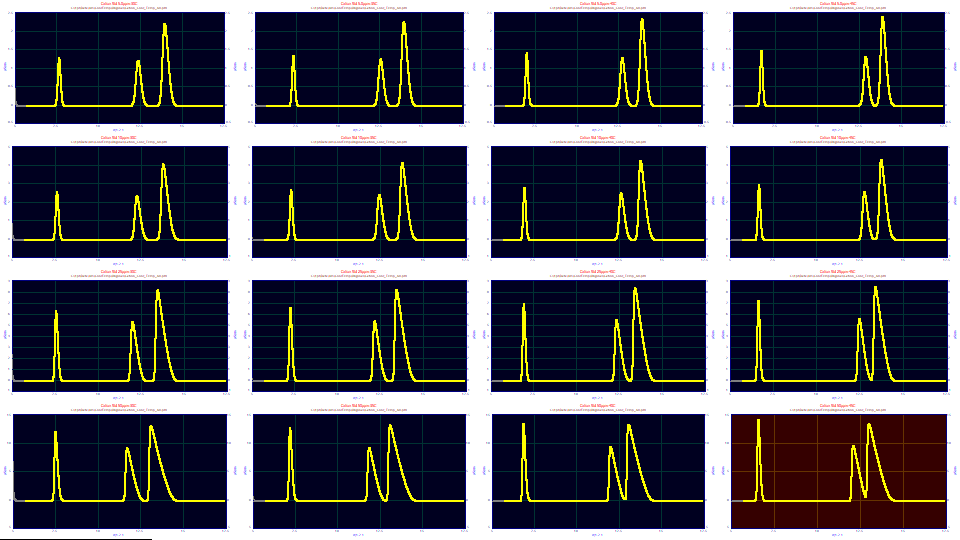
If we fit the GenNLC<ge> to just the tailed peaks, with the a4 locked to the same 1.2082 ZDD asymmetry, and a7 locked to the .625 area fraction of the narrow IRF component, we see the following when all sixteen data sets are averaged:
AverageĀforĀ16ĀFits
FittedĀParameters
r2ĀĀCoefĀDetĀ DFĀAdjĀr2ĀĀ FitĀStdĀErrĀ F-valueĀ ppmĀuVar
0.99996608Ā 0.99996602Ā 0.00932128Ā 20,179,722Ā 33.9214551
ĀPeakĀ TypeĀĀĀĀĀĀĀĀ ĀĀĀa0ĀĀĀĀĀĀ ĀĀĀa1ĀĀĀĀĀĀĀ ĀĀĀa2ĀĀĀĀĀĀ ĀĀĀĀa3ĀĀĀĀĀĀ ĀĀĀĀa4ĀĀĀĀĀ ĀĀĀa5ĀĀĀĀĀĀĀ ĀĀĀĀa6ĀĀĀĀĀ ĀĀĀĀa7ĀĀĀĀĀ
ĀĀĀĀ1Ā GenNLC<ge>ĀĀ 1.21997308Ā 7.11478834ĀĀ 0.00037890Ā 0.00169294ĀĀ 1.20820000Ā 0.01751915ĀĀ 0.04459583Ā 0.62500000ĀĀ
ĀĀĀĀ2Ā GenNLC<ge>ĀĀ 2.07707881Ā 12.6113183ĀĀ 0.00076753Ā 0.01243254ĀĀ 1.20820000Ā 0.01751915ĀĀ 0.04459583Ā 0.62500000ĀĀ
ĀĀĀĀ3Ā GenNLC<ge>ĀĀ 4.21419000Ā 14.1015128ĀĀ 0.00088205Ā 0.02821404ĀĀ 1.20820000Ā 0.01751915ĀĀ 0.04459583Ā 0.62500000ĀĀ
This match with the fronted peaks estimate for the exponential term may be due to the sixth peak with the largest area predominating in the fitting. The narrow width component fitted to almost twice the half-Gaussian SD observed when the fronted peaks were included in the fit.
If we refit with these values and allow a5 and a6 to vary, as we did when fitting all peaks, we can again average the 14 sets for the K+ peak and the 8 sets for Ca+ and Mg+ peaks:
Peak 1: Potassium
AverageĀforĀ14ĀFits
FittedĀParameters
r2ĀĀCoefĀDetĀ DFĀAdjĀr2ĀĀ FitĀStdĀErrĀ F-valueĀ ppmĀuVar
0.99997755Ā 0.99997750Ā 0.00664231Ā 23,650,255Ā 22.4514665
ĀPeakĀ TypeĀĀĀĀĀĀĀĀ ĀĀĀa0ĀĀĀĀĀĀ ĀĀĀa1ĀĀĀĀĀĀĀ ĀĀĀa2ĀĀĀĀĀĀ ĀĀĀĀa3ĀĀĀĀĀĀ ĀĀĀĀa4ĀĀĀĀĀ ĀĀĀa5ĀĀĀĀĀĀĀ ĀĀĀĀa6ĀĀĀĀĀ ĀĀĀĀa7ĀĀĀĀĀ
ĀĀĀĀ1Ā GenNLC<ge>ĀĀ 1.00811700Ā 7.06420650ĀĀ 0.00036583Ā 0.00113221ĀĀ 1.20820000Ā 0.01302649ĀĀ 0.05164986Ā 0.62500000Ā
ĀĀĀĀ2Ā GenNLC<ge>ĀĀ 1.71314332Ā 12.6582763ĀĀ 0.00077087Ā 0.01025646ĀĀ 1.20820000Ā 0.00945635ĀĀ 0.02333329Ā 0.62500000Ā
ĀĀĀĀ3Ā GenNLC<ge>ĀĀ 3.47345967Ā 14.1050224ĀĀ 0.00089319Ā 0.02319855ĀĀ 1.20820000Ā 0.00708538ĀĀ 0.02966004Ā 0.62500000
Peak 2: Calcium, Peak 3: Magnesium
AverageĀforĀ8ĀFits
FittedĀParameters
r2ĀĀCoefĀDetĀ DFĀAdjĀr2ĀĀ FitĀStdĀErrĀ F-valueĀ ppmĀuVar
0.99997286Ā 0.99997280Ā 0.01309497Ā 19,070,879Ā 27.1416789
ĀPeakĀ TypeĀĀĀĀĀĀĀĀ ĀĀĀa0ĀĀĀĀĀĀ ĀĀĀa1ĀĀĀĀĀĀĀ ĀĀĀa2ĀĀĀĀĀĀ ĀĀĀĀa3ĀĀĀĀĀĀ ĀĀĀĀa4ĀĀĀĀĀ ĀĀĀa5ĀĀĀĀĀĀĀ ĀĀĀĀa6ĀĀĀĀĀ ĀĀĀĀa7ĀĀĀĀĀ
ĀĀĀĀ1Ā GenNLC<ge>ĀĀ 2.03869919Ā 7.11508092ĀĀ 0.00038183Ā 0.00278430ĀĀ 1.20820000Ā 0.01549019ĀĀ 0.04444166Ā 0.62500000Ā
ĀĀĀĀ2Ā GenNLC<ge>ĀĀ 3.46253250Ā 12.5467267ĀĀ 0.00072935Ā 0.02020250ĀĀ 1.20820000Ā 0.02119142ĀĀ 0.05395209Ā 0.62500000Ā
ĀĀĀĀ3Ā GenNLC<ge>ĀĀ 7.02981958Ā 14.1154983ĀĀ 0.00093258Ā 0.04690051ĀĀ 1.20820000Ā 0.01265206ĀĀ 0.04339503Ā 0.62500000
Fitting Only Tailed Peaks
Fitting Both Tailed And Fronted Peaks
[0.01302649, 0.05164986]
[0.01314113, 0.05167537]
[0.02119142, 0.05395209]
[0.02115366, 0.05390487]
[0.01265206, 0.04339503]
[0.01267363, 0.04340435]
If we compare the independent values of the tailed fits with and without the fronted peaks in the data, the results are nearly identical. The values for three different +a3 tailed peaks, however, vary far more than was observed with the three -a3 fronted peaks.
We will be exploring the genetic algorithm in the IRF Deconvolution procedure with this first of these tailed peaks. With this separate analysis, we expect this K+ peak to fit to about 0.052 exponential width and 0.013 half-Gaussian width. The other two tailed peaks elute too closely together and most data sets lack a baseline between these two peaks, a requirement for the IRF Deconvolution genetic algorithm to be effective.
IRF Deconvolution using a Genetic Algorithm Optimization
If the correlation between the IRF and an intrinsic tailed shape causes the fitting a GenHVL<irf> or GenNLC<irf> model to be consistently overspecified even when locking the ZDD asymmetry and IRF component fractions, there may be an alternative. The Fourier IRF Deconvolution procedure offers a genetic algorithm optimization that seeks to maximize the amount of baseline after the deconvolution of the IRF.
If you look closely at an IRF deconvolution you will see that too weak of an IRF results in the deconvolved peak failing to decay fully to the baseline. If the IRF is too strong, the deconvolved peak will produce an oscillation that falls below the baseline, to negative values. By maximizing the amount of baseline, a good approximation to the IRF is realized.
The main difficulty with this approach on two component IRFs is that nearly all of the tailing rests with the higher width exponential component. If we isolate only this first of the three tailed peaks and use the genetic algorithm locking the .625 area fraction (vary 0%) and allowing the half-Gaussian SD to vary 0.01 ▒ 50% and the exponential width to vary 0.05 ▒ 50%, optimizing the BsLnZero procedure with a 0.5% tolerance for the baseline produces the following:
IRF ĀParmĀ1ĀĀĀ ParmĀ2ĀĀĀ ParmĀ3
<ge> 0.0050000 0.0476503 0.6250000 CationStdĀ 5ppm 30C
<ge> 0.0050000 0.0542916 0.6250000 CationStdĀ 5ppm 35C
<ge> 0.0050000 0.0525535 0.6250000 CationStdĀ 5ppm 40C
<ge> 0.0050000 0.0469912 0.6250000 CationStdĀ 5ppm 45C
<ge> 0.0050000 0.0562200 0.6250000 CationStdĀ 10ppm 30C
<ge> 0.0050000 0.0517323 0.6250000 CationStdĀ 10ppm 35C
<ge> 0.0050000 0.0508961 0.6250000 CationStdĀ 10ppm 40C
<ge> 0.0050000 0.0476099 0.6250000 CationStdĀ 10ppm 45C
<ge> 0.0050000 0.0560884 0.6250000 CationStdĀ 25ppm 30C
<ge> 0.0050000 0.0536355 0.6250000 CationStdĀ 25ppm 35C
<ge> 0.0050000 0.0504921 0.6250000 CationStdĀ 25ppm 40C
<ge> 0.0050000 0.0498951 0.6250000 CationStdĀ 25ppm 45C
<ge> 0.0050000 0.0588461 0.6250000 CationStdĀ 50ppm 30C
<ge> 0.0050000 0.0573139 0.6250000 CationStdĀ 50ppm 35C
<ge> 0.0050000 0.0547953 0.6250000 CationStdĀ 50ppm 40C
<ge> 0.0050000 0.0511005 0.6250000 CationStdĀ 50ppm 45C
The Half-Gaussian iterated to the lower bound in all of the optimizations. The average exponential width optimized to .0525 (we saw .0516 on the fits for this K+ peak when separate widths were fitted).
The above procedure works well for fronted peaks. For tailed peaks, there is a more sophisticated genetic optimization. We can look at the fits for the K+ peak and see that the IRF attenuates the peak by a certain measure. If you look at the amplitudes in the Numeric Summary for the K+ peak, we see about 1.10x higher amplitude in the deconvolution. The AmpAtten algorithm will isolate the parameters in the vicinity of this 1.10x and optimize those for this maximum baseline. If we again lock the .625 area fraction and allow the half-Gaussian SD to vary 0.01 ▒ 50% and the exponential width to vary 0.05 ▒ 50%, optimizing the AmpAtten procedure with a 1.10% amplitude factor, we see the following:
IRF ĀParmĀ1ĀĀĀ ParmĀ2ĀĀĀ ParmĀ3
<ge> 0.0069547 0.0565495 0.6250000 CationStdĀ 5ppm 30C
<ge> 0.0064012 0.0591251 0.6250000 CationStdĀ 5ppm 35C
<ge> 0.0056325 0.0566471 0.6250000 CationStdĀ 5ppm 40C
<ge> 0.0055000 0.0522448 0.6250000 CationStdĀ 5ppm 45C
<ge> 0.0061659 0.0614142 0.6250000 CationStdĀ 10ppm 30C
<ge> 0.0115644 0.0575498 0.6250000 CationStdĀ 10ppm 35C
<ge> 0.0140587 0.0571281 0.6250000 CationStdĀ 10ppm 40C
<ge> 0.0055000 0.0534846 0.6250000 CationStdĀ 10ppm 45C
<ge> 0.0124300 0.0575157 0.6250000 CationStdĀ 25ppm 30C
<ge> 0.0127802 0.0554683 0.6250000 CationStdĀ 25ppm 35C
<ge> 0.0115247 0.0539039 0.6250000 CationStdĀ 25ppm 40C
<ge> 0.0141052 0.0528506 0.6250000 CationStdĀ 25ppm 45C
<ge> 0.0085685 0.0517043 0.6250000 CationStdĀ 50ppm 30C
<ge> 0.0122042 0.0510394 0.6250000 CationStdĀ 50ppm 35C
<ge> 0.0107607 0.0495663 0.6250000 CationStdĀ 50ppm 40C
<ge> 0.0133762 0.0491243 0.6250000 CationStdĀ 50ppm 45C
The sixteen peaks average 0.00985 and 0.0547 for the two parameters.
The AmpAtten algorithm will strongly bind the principal tailing component, the exponential, but not the narrow width component. You can use this procedure as a second check on the constrained fits. Simply enter the amplitude factor for the deconvolution in the fit. You may or may not see this genetic optimization recover the parameters of the fits. Here there is no inter-correlation between the tailed intrinsic chromatographic shape and the tailing in the IRF. There is only the raw data, an expectation of the amplitude change arising from the deconvolution of the IRF, and a maximization of baseline within a narrow zone around that measure of sharpened amplitude.
The Wider Exponential Component
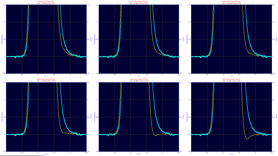
The above plots are of a series of zoomed-in deconvolutions with where the half-Gaussian width is set to the 0.009 and the narrow width fraction is set to .625. The exponential width varies .040, .044, .048, .052, .056, and .060. The exponential component's impact on the tailing is so prominent you can actually do a manual deconvolution optimization on this parameter (with the others locked). Here the optimum exponential would be seen as occurring between the .052 of the fourth graph and the .056 of the fifth.
The Narrow Width Component
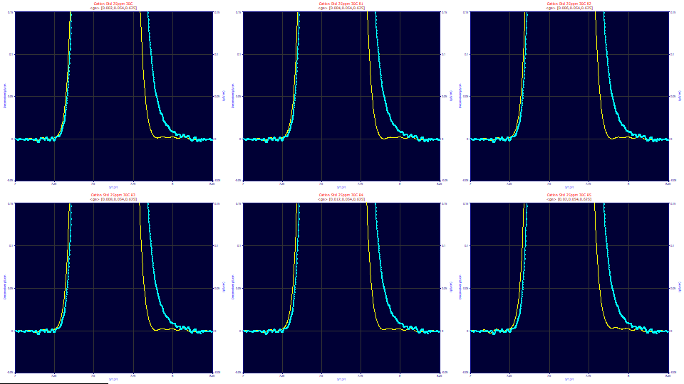
The above plots are of a series of zoomed-in deconvolutions with where the exponential width is set to the 0.054 and the narrow width fraction is set to .625. The narrow width varies .002, .004, .006, .008, .012, and .020. The narrow width component's impact on the tailing is very subtle. Note also the oscillations around the baseline. This is why a genetic optimization is needed, and why the estimate of this narrow component is difficult. Both the data and the Fourier-filtered deconvolution are noisy and oscillating if you look closely at the baseline.
An IRF is an average of the instrumental and system distortions which alter the true shape of the chromatographic peak. The average parameters within an IRF may vary with the species and with the location of its elution. Further, it is likely that even a two-component IRF is an approximation of a series of complex processes which can perhaps be described sufficiently with a basic two-component model, but where those parameters may not be absolutely constant. This appears to be the case for the narrow component, but it may be that the narrow parameter is simply far harder to estimate since its tailing is mostly masked by the tailing of the much wider exponential. And as we noted in this example, be cautious of blind averaging. IRF parameters can iterate to zero and such fits should be excluded from any IRF averaging.
Estimating an IRF with only tailed peaks is certainly possible, and we appreciate there may well be instances where such is necessary. The procedures outlined in this topic should help get you a respectable estimate.
We will cover one more instance of estimating a tailed peak IRF. We will address the very different IRF shapes which occur with GC peaks.
Ā
Ā


 |