PeakLab v1 Documentation Contents AIST Software Home AIST Software Support
IRF Estimation 2 - Standards Sectioned to Contain Only 'Fronted' Peaks
In this second approach to estimating an IRF, we will use the same standard as in the IRF Estimation 1 approach, but we will section the data to fit only the first fronted peak in the 5, 10, and 25 ppm standards.

The Problem with Tailed Peaks and IRF Estimation
We will begin by looking at the IRF fits in the IRF Estimation 1 example, and plot the most fronted and tailed peaks in one of the 25 ppm concentration fits:
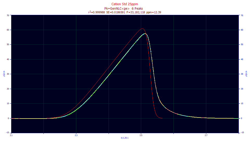
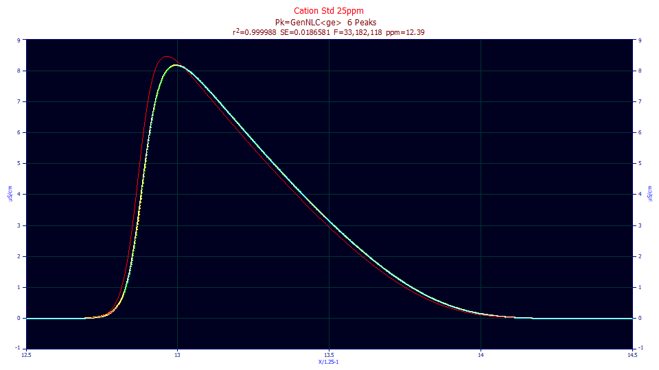
The red curve is the IRF-deconvolved fit, the fit determined by the parameters absent the IRF component. The red is thus the peak that would be seen if no IRF were present; that is, the instrument smears the red curve into the peak that appears in the data. For the fronted peak, because the skew of the peak and the skew of the IRF are in opposite directions, and because fronted peaks are often the earliest to elute and thus narrower in width, there tends to be a sharp difference between the peak with and without the IRF. For the tailed peak, the skew of the peak and the skew of the IRF are in the same direction, and further, strongly tailed peaks are often the last to elute and thus of a greater width. The difference between the peak with and without the IRF is much less.
In statistical terms, the IRF and tailed peak parameters are more likely to be correlated, each somewhat indistinguishable from one another in their impact upon the model. In other words, the tailing of the IRF blends in with the tailing of native peak. When the two are almost indistinguishable as in the plot above, the fit algorithm will have difficulty resolving the parameters for the two different tailing processes.
Fitting Only the Most Fronted Peak with the GenNLC<ge> Model
Just as one can generally safely assume the IRF will be close to constant across concentration, one can usually assume the IRF is constant across time within the chromatogram, whether a peak is strongly fronted, narrow, and the first peak to appear, or strongly tailed, wide, and the last peak to appear.
In this estimation, we will isolate the first eluting peak in the standard used in the IRF Estimation 1 example and fit the same nine data sets (three series across time at 5, 20, and 25 ppm concentration) to the GenNLC<ge> model:
Averageаforа9аFits
FittedаParameters
r2аCoefаDetаа DFаAdjаr2аааа FitаStdаErrаа F-valueаааааа ppmаuVar
0.99999486ааа 0.99999482ааа 0.01852498ааа 35,613,035ааа 5.13756651
аPeakаа Typeаааааааа ааааааa0аааа ааааааa1аааа ааааааa2аааа ааааааa3аааа ааааааa4аааа ааааааa5аааа ааааааa6аааа ааааааa7аааа
аааа1аа GenNLC<ge>аа 4.71457477аа 2.31818277аа 0.00024211аа -0.0059113аа 1.17888115аа 0.00681811аа 0.04313462аа 0.62990383аа
CVаPercentаforа9аFits
FittedаParameters
r2аCoefаDetаа DFаAdjаr2аааа FitаStdаErrаа F-valueаааааа ppmаuVar
0.00032206ааа 0.00032450ааа 78.6187622ааа 33.7527815ааа 62.6876684
аPeakаа Typeаааааааа ааааааa0аааа ааааааa1аааа ааааааa2аааа ааааааa3аааа ааааааa4аааа ааааааa5аааа ааааааa6аааа ааааааa7аааа
аааа1аа GenNLC<ge>аа 67.4922715аа 0.94823526аа 4.45440137аа 66.1591631аа 12.0786590аа 52.1341809аа 0.75540920аа 3.02022061аа
The values we estimated for the <ge> IRF in the the IRF Estimation 1 example were [0.0080, 0.04316, 0.621]. Here we have almost exactly the same 'e' exponential tau, and the same area fraction for the Gaussian. The average half-Gaussian response width, however, is somewhat less. Let's look at this data differently and also average the three 5, 10, and 25 ppm fits:
Averageаforаthreeа5аppmаFits
FittedаParameters
r2аCoefаDetаа DFаAdjаr2аааа FitаStdаErrаа F-valueаааааа ppmаuVar
0.99999565ааа 0.99999561ааа 0.00731264ааа 35,938,653ааа 4.35397757
аPeakаа Typeаааааааа ааааааa0аааа ааааааa1аааа ааааааa2аааа ааааааa3аааа ааааааa4аааа ааааааa5аааа ааааааa6аааа ааааааa7аааа
аааа1аа GenNLC<ge>аа 1.77347599аа 2.33957221аа 0.00024529аа -0.0022722аа 1.13489593аа 0.00309406аа 0.04319880аа 0.63763542аа
CVаPercentаforаthreeа5аppmаFits
FittedаParameters
r2аCoefаDetаа DFаAdjаr2аааа FitаStdаErrаа F-valueаааааа ppmаuVar
9.7136e-5аааа 9.788e-5ааааа 9.99223089ааа 19.8595198ааа 22.3120398
аPeakаа Typeаааааааа ааааааa0аааа ааааааa1аааа ааааааa2аааа ааааааa3аааа ааааааa4аааа ааааааa5аааа ааааааa6аааа ааааааa7аааа
аааа1аа GenNLC<ge>аа 0.93539385аа 0.54395807аа 2.30976597аа 1.25213762аа 22.6172011аа 140.114352аа 1.21257714аа 5.31354888а
Averageаforаthreeа10аppmаFits
FittedаParameters
r2аCoefаDetаа DFаAdjаr2аааа FitаStdаErrаа F-valueаааааа ppmаuVar
0.99999587ааа 0.99999584ааа 0.01328945ааа 39,256,195ааа 4.12542900
аPeakаа Typeаааааааа ааааааa0аааа ааааааa1аааа ааааааa2аааа ааааааa3аааа ааааааa4аааа ааааааa5аааа ааааааa6аааа ааааааa7аааа
аааа1аа GenNLC<ge>аа 3.53759334аа 2.32080542аа 0.00022951аа -0.0044967аа 1.25229684аа 0.00855179аа 0.04324721аа 0.62334698аа
CVаPercentаforаthreeа10аppmFits
FittedаParameters
r2аCoefаDetаа DFаAdjаr2аааа FitаStdаErrаа F-valueаааааа ppmаuVar
0.00012923ааа 0.00013019ааа 14.5424412ааа 30.3054744ааа 31.3228332
аPeakаа Typeаааааааа ааааааa0аааа ааааааa1аааа ааааааa2аааа ааааааa3аааа ааааааa4аааа ааааааa5аааа ааааааa6аааа ааааааa7аааа
аааа1аа GenNLC<ge>аа 1.18737301аа 0.41425904аа 0.82651015аа 0.40048571аа 4.28786134аа 6.68955456аа 0.45352651аа 1.59413959аа
Averageаforаthreeа25аppmаFits
FittedаParameters
r2аCoefаDetаа DFаAdjаr2аааа FitаStdаErrаа F-valueаааааа ppmаuVar
0.99999307ааа 0.99999301ааа 0.03497286ааа 31,644,258ааа 6.93329297
аPeakаа Typeаааааааа ааааааa0аааа ааааааa1аааа ааааааa2аааа ааааааa3аааа ааааааa4аааа ааааааa5аааа ааааааa6аааа ааааааa7аааа
аааа1аа GenNLC<ge>аа 8.83265496аа 2.29417067аа 0.00025151аа -0.0109652аа 1.14945069аа 0.00880847аа 0.04295784аа 0.62872909аа
CVаPercentаforаthreeа25аppmаFits
FittedаParameters
r2аCoefаDetаа DFаAdjаr2аааа FitаStdаErrаа F-valueаааааа ppmаuVar
0.00056198ааа 0.00056621ааа 41.3070800ааа 58.4231917ааа 81.0544013
аPeakаа Typeаааааааа ааааааa0аааа ааааааa1аааа ааааааa2аааа ааааааa3аааа ааааааa4аааа ааааааa5аааа ааааааa6аааа ааааааa7аааа
аааа1аа GenNLC<ge>аа 0.93954335аа 0.47140661аа 2.62973527аа 0.03698853аа 0.60398245аа 4.60720109аа 0.46421850аа 1.06490869аа
While the 10 ppm and 25 ppm fits have closer to the 0.008 'g' width we found in fitting all six peaks in the standard and averaging across samples and concentrations, here the 'g' for the 5 ppm samples averages to just .003. Given the fit to just a single peak, and the lower S/N and lower chromatographic distortion on the 5 ppm sample, the 0.008 of the higher S/N and higher a3 samples is likelier correct.
Confirmation with Fourier Deconvolution
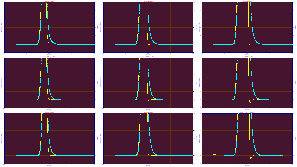
If we enter the .0087, .0431, and .625 from the 10 and 25 ppm averages in the IRF Deconvolution option and zoom in on the first peak, we see the following:
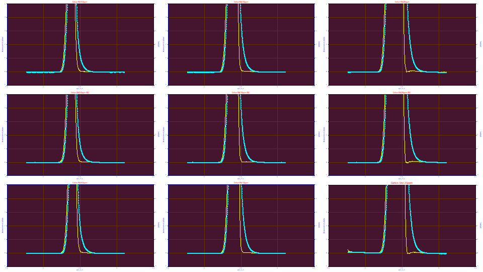
The Fourier deconvolution across all nine data sets, using these <ge> parameters, zoomed in for the first peak, isn't perfect across all nine sets, but it is close. If we enter .003 for the 'g' SD, from the 5 ppm fits, the deconvolution errors in the plots above are clearly greater, and is especially obvious with the 25 ppm concentration:
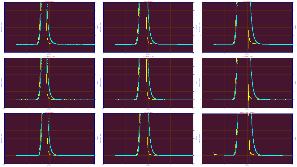
If we enter .015 for the 'g' SD, we see an incomplete deconvolution at the 5 and 10 ppm concentration, and a clear breakdown in the deconvolution on the 25 ppm concentration samples.
When one is having difficulty consistently fitting an IRF, inspection of the different parameters in a Fourier deconvolution helps visualize what is happening. The IRF Deconvolution procedure also offers a genetic algorithm which will seek to optimize an IRF by maximizing the amount of baseline.
An IRF Models System Effects Which May Not Be Truly Constant
As evident here in these single peak fits, an IRF may model system effects which vary somewhat with sample concentrations, temperature, additives, and other prep or run factors. The 'g' component in this example is not the 'primary' component of the IRF, even though it represents better than half the overall IRF on an area basis. There is a significant amount of this probabilistic distortion occurring, but its impact on the overall peak shape is much less because it is quite small in width. This secondary 'g' component may be modeling system nonidealities which are not absolutely constant, such as axial dispersion. In such cases, you will want a good average of this 'g' component accepting that a certain compromise will be necessary to assume a constant IRF.
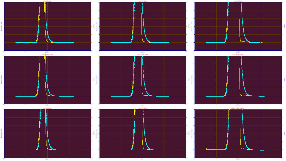
Again, the Fourier Deconvolution option furnishes a near immediate cross check of the validity of the IRF before removing it. In the above example, we approximately halved and doubled the 'g' component's width. In varying 'g' one observes only slowly changing effects. Let us now visually adjust this much larger and highly constant primary 'e' component. Let us reduce 'e' from 0.428 to 0.418. Clearly the width is now too small.
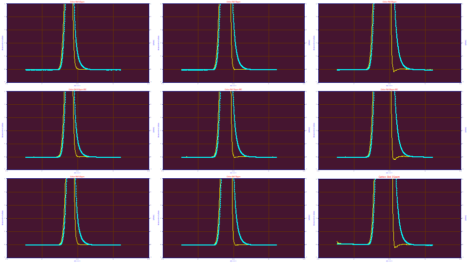
Let us now increase 'e' from 0.428 to 0.438. Clearly the width is too large. The larger width in an IRF is actually this sensitive in a deconvolution and rather easily visualized.
A fronted peak is preferable for this genetic algorithm estimation of the IRF estimation since it exhibits this lovely transition at the baseline. While we will not say that this genetic procedure fails with tailed peaks, we can note it is harder. If you can manage it, you may want to add an early eluting fronted peak to your standard specifically for instrumental modeling. Please remember that if you do this and the peak appears tailed, it may actually be fronted and the tailing you see is from the instrumental distortion. You will need to fit such a peak to be certain.
Fitting Only the Most Fronted Peak with the GenNLC<e2> Model
Averageаforа9аFits
FittedаParameters
r2аCoefаDetаа DFаAdjаr2аааа FitаStdаErrаа F-valueаааааа ppmаuVar
0.99999562ааа 0.99999558ааа 0.01740951ааа 41,476,901ааа 4.38248857
аPeakаа Typeаааааааа ааааааa0аааа ааааааa1аааа ааааааa2аааа ааааааa3аааа ааааааa4аааа ааааааa5аааа ааааааa6аааа ааааааa7аааа
аааа1аа GenNLC<e2>аа 4.71548080аа 2.31799021аа 0.00024086аа -0.0059039аа 1.24802205аа 0.00561802аа 0.04377159аа 0.63718806аа
CVаPercentаforа9аFits
FittedаParameters
r2аCoefаDetаа DFаAdjаr2аааа FitаStdаErrаа F-valueаааааа ppmаuVar
0.00032834ааа 0.00033098ааа 83.5864512ааа 37.0837027ааа 74.9193363
аPeakаа Typeаааааааа ааааааa0аааа ааааааa1аааа ааааааa2аааа ааааааa3аааа ааааааa4аааа ааааааa5аааа ааааааa6аааа ааааааa7аааа
аааа1аа GenNLC<e2>аа 67.4956866аа 0.83754286аа 4.98583029аа 65.6072824аа 9.92539336аа 6.856777526аа 0.61770387аа 2.845947898
In this instance the <e2> IRF has no issue at the 5 ppm concentration. You should not automatically assume that a two-exponential IRF is going to be more correlated, and less stable, than the sum of the half-Gaussian and exponential IRF. It is quite possible a fast and slow kinetic distortion is a more accurate picture of a system's distortions. Here we see the same .437 slow 'e' and it has close to the same area fraction as the <ge> IRF. Here the fast 'e' is .0056, and stable, with only a 6.85% CV across the nine fits of the one fronted peak.
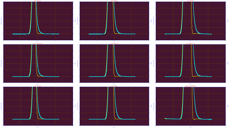
Again, we suspect the fast component of both the <e2> and <ge> distortions is probably modeling a mix of kinetic and probabilistic non-idealities, and why each of these IRFs appear about equally viable in many of the data sets where we've done IRF determinations.
In this example, the <e2> IRF looks slightly more stable then the <ge> across the different samples and concentrations in this deconvolution visualization.
Solvent or System Peaks
In many chromatograms, there may be a ready made early eluting peak in the form of a solvent or system peak which appears just after the column dead time. In our experience, such peaks may appear tailed, but because of there being virtually no chromatographic separation, are probably absent any a3 chromatographic fronting or tailing. Nearly the whole of the tailing should be from the IRF.
The non-retained peak at the dead-time has no chromatographic separation and fitting a model based upon such is dubious, although the GenHVL and GenNLC models will adjust for the lack of chromatographic distortion (a3 iterating to near 0). We have been successful in fitting a clean dead time peak, even though such will be a mix of all unretained components. We were able to get the higher width exponential correct, but the narrow width component often iterated to zero. The bigger problem in using the unretained peak for IRF estimation is that it is not a single entity, everything unretained is there, and certain impurities may be ever so slightly retained distorting this t0 shape. Further, in the event of IC, those different unretained components may have different ionic charges resulting in anything but a coherent peak.
As such, you may wish to consider fitting a peak with a tiny measure of chromatographic separation that occurs immediately after the dead-time pulse, if such exists.
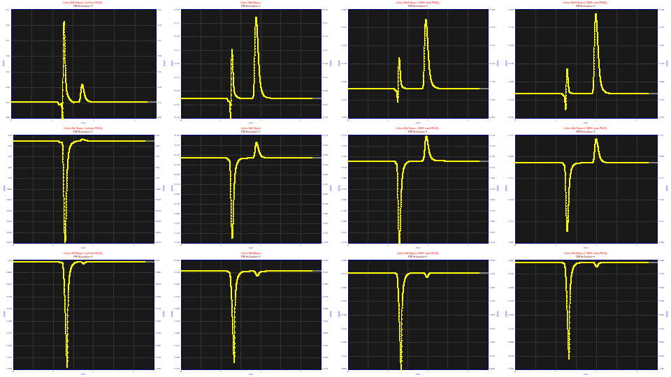
Here are the solvent/system peaks in the data series we have been using for these various IRF estimation examples. There is a second peak following the t0 peak that is unrelated to concentration of the solutes. There is the t0 peak which is not cleanly defined in any of the runs, but which can possibly be fitted in the 10 ppm and 25 ppm concentration data sets in the second and third rows in the plot above.
We simply proceed as if these were solute peaks, reversing the sign of the signal where needed, performing a baseline subtraction, and then transforming for the t0=1.15 dead time.
Fitting Peak Just After t0 with the GenNLC<e> Model
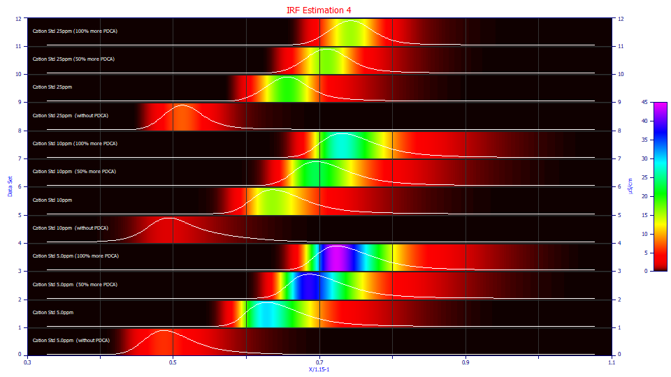
If we look at only this post-dead-time peak in the View and Compare Data option using a contour with no area or amplitude normalization, we see that the the samples without the PDCA additive have a much smaller magnitude second peak and these elute sooner. The samples with PDCA elute later, and the greater the PDCA amount in the prep, the later the elution. The magnitude of the peak is strongly correlated with the amount of PDCA on the 5 ppm samples. The 10 ppm samples have this same trend, do not evidence a higher measure of broadening, and are lower in overall magnitude. This peak on the 25 ppm samples is actually less broadened and for the higher PDCA concentrations, is even smaller in magnitude. In all cases, if you look closely at the contours and peak shapes, there is a tailing in the peaks as they are registered by the instrument.
We have been suitably warned. A peak which is clearly related to additive concentration, in both location and magnitude, exists when no additive is present. The peak also narrows and decreases in magnitude with higher concentration. If there are two (or more) components mixed within this post t0 peak, any IRF estimation will be suspect.
In order to get fits that are useful on such peaks, we must either fit the NLC<ge> model (absent the ZDD asymmetry adjustment for the third moment), or we must lock this a4 asymmetry (third moment ZDD adjustment) parameter at a value typical of the GenNLC<ge> model. We will do the latter, setting the a4 asymmetry to the program's default of 1.186. This locked value, which is somewhat higher than the Giddings' 0.5 asymmetry in the NLC, is used to constrain the ZDD of these fits to values traditionally seen with such models. One of the GenNLC<ge> peaks had an anomalous shape and a weak fit, and was omitted from the average.
Averageаforа11аFits
FittedаParameters
r2аCoefаDetаа DFаAdjаr2аааа FitаStdаErrаа F-valueаааааа ppmаuVar
0.99997517ааа 0.99997483ааа 0.01808092ааа 14,749,422ааа 24.8323020
аPeakаа Typeаааааааа ааааааa0аааа ааааааa1аааа ааааааa2аааа ааааааa3аааа ааааааa4аааа ааааааa5аааа ааааааa6аааа ааааааa7аааа
аааа1аа GenNLC<ge>аа 2.03591564аа 0.66395635аа 0.00062278аа 0.00202550аа 1.18580000аа 0.00680595аа 0.04652329аа 0.61186396аа
CVаPercentаforа11аFits
FittedаParameters
r2аCoefаDetаа DFаAdjаr2аааа FitаStdаErrаа F-valueаааааа ppmаuVar
0.00265098ааа 0.00268737ааа 41.4368373ааа 102.472614ааа 106.752769
аPeakаа Typeаааааааа ааааааa0аааа ааааааa1аааа ааааааa2аааа ааааааa3аааа ааааааa4аааа ааааааa5аааа ааааааa6аааа ааааааa7аааа
аааа1аа GenNLC<ge>аа 62.0529065аа 14.0095544аа 15.8265837аа 115.358597аа 0.00000000аа 98.9459839аа 15.9917944аа 15.7660537аа
If you have been following the previous three examples, we realized an IRF of [0.0080, 0.0432, 0.621] from fitting all fronted and tailed peaks in these standards (IRF Estimation 1) , [0.0087, 0.0431, 0.625] from fitting the first fronted peak in these standards. Our average IRF here of [0.0068, 0.0465, 0.612] is surprisingly close. The CV percents are high as compared to the solute peaks, suggesting many more such system peaks would wisely be averaged in order to arrive at a sound estimate of the IRF.
The a3 did fit to a tailed shape.
Fitting the t0 'Mash' with the GenNLC<ge> Model
At this point, we will fit the mash of everything that elutes at the dead time volume, that which is nowhere retained. Here we must use only the 10 and 25 ppm samples since the the 5 ppm peaks oscillated about the baseline, certainly suggestive of various components with different ionic charges.
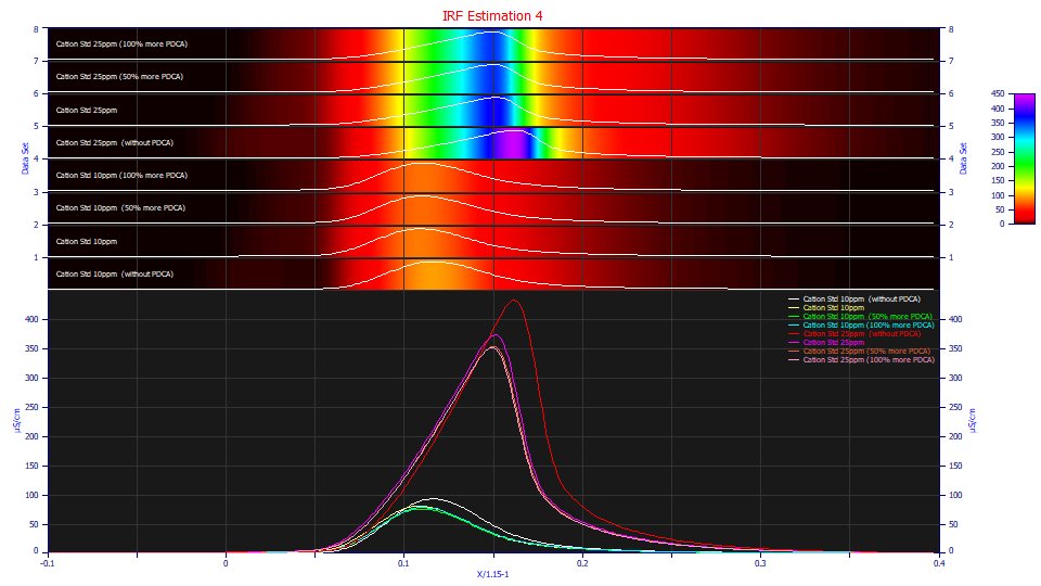
Although none of the eight t0 peaks are clean in their rise, and there are differences between additive-bearing and non-additive runs, the additive influence is much less. We also see the familiar indeterminate shape we described in the IRF Estimation 1 example for a fronted peak that appears tailed as a consequence of the tailing in the IRF.
These fits are poorer, as expected from the visible perturbation that occurs near the t0 rise of the peak, as well as the mix of components lumped into this one peak. Such a peak whose component ionic charges and locations are such that the 5 ppm samples are unfittable due to having an oscillating signal instead of peak, should be considered a last resort in an IRF estimation.
Averageаforа8аFits
FittedаParameters
r2аCoefаDetаа DFаAdjаr2аааа FitаStdаErrаа F-valueаааааа ppmаuVar
0.99974842ааа 0.99974462ааа 0.68344060ааа 366,073аааааа 251.575019
аPeakаа Typeаааааааа ааааааa0аааа ааааааa1аааа ааааааa2аааа ааааааa3аааа ааааааa4аааа ааааааa5аааа ааааааa6аааа ааааааa7аааа
аааа1аа GenNLC<ge>аа 16.4734538аа 0.10436431аа 0.00212077аа -0.0146913аа -0.0718759аа 0.00272253аа 0.04477119аа 0.79476011аа
CVаPercentаforа8аFits
FittedаParameters
r2аCoefаDetаа DFаAdjаr2аааа FitаStdаErrаа F-valueаааааа ppmаuVar
0.01161848ааа 0.01179423ааа 53.5207178ааа 45.6786505ааа 46.1713533
аPeakаа Typeаааааааа ааааааa0аааа ааааааa1аааа ааааааa2аааа ааааааa3аааа ааааааa4аааа ааааааa5аааа ааааааa6аааа ааааааa7аааа
аааа1аа GenNLC<ge>аа 67.9831477аа 13.3472578аа 6.23123076аа 161.064853аа 255.892590аа 100.667339аа 6.25773213аа 26.3491419аа
If we compare this [0.0027, 0.0448, .794] IRF estimate with the [0.0080, 0.0432, 0.621], [0.0087, 0.0431, 0.625], of the other estimations, and the [0.0068, 0.0465, 0.612] from this second system peak, we can't be particularly encouraged, but the stability of the a6 'e' exponential parameter is impressive.
In the instance of the data used in all of these IRF Estimation examples, there was never an instance where any single exponential model (GenNLC<e> or NLC<e>) successfully fit the IRF. We have, in fact, never seen a chromatographic data set, LC or GC, where a simple exponential model accurately modeled the IRF. We furnish an <e> IRF model, for noisy data and for the instances of very slow detectors where the exponential response overrides all else.
When fitting the t0 unretained peak, and wanting to improve the variability in the estimated parameters, one might wish to try the simpler NLC<ge> model where the intrinsic zero-distortion density's asymmetry is locked at the Giddings of the pure NLC model, or perhaps lock the GenNLC a4 at a specific asymmetry. If you do this, look closely at the degradation in the goodness of fit. The asymmetry in the generalized model may well be accommodating different components that make up this unretained peak. In other words, an odd asymmetry, positive or negative, is likely from the mix of unretained components.
For example, here is this same fit of this t0 peak to this simpler NLC<ge> model:
Averageаforа8аFits
FittedаParameters
r2аCoefаDetаа DFаAdjаr2аааа FitаStdаErrаа F-valueаааааа ppmаuVar
0.99902472ааа 0.99901184ааа 1.81627818ааа 148,354аааааа 975.279214
аPeakаа Typeаааааааа ааааааa0аааа ааааааa1аааа ааааааa2аааа ааааааa3аааа ааааааa4аааа ааааааa5аааа ааааааa6аааа ааааааааа
аааа1аа NLC<ge>аа 16.3183264аа 0.10099324аа 0.00193297аа -0.0067235аа 0.00145546аа 0.04513449аа 0.65620302аа
CVаPercentаforа8аFits
FittedаParameters
r2аCoefаDetаа DFаAdjаr2аааа FitаStdаErrаа F-valueаааааа ppmаuVar
0.06572511ааа 0.06659403ааа 87.2424546ааа 69.4973578ааа 67.3253413
аPeakаа Typeаааааааа ааааааa0аааа ааааааa1аааа ааааааa2аааа ааааааa3аааа ааааааa4аааа ааааааa5аааа ааааааa6аааа аааааааааа
аааа1аа NLC<ge>аа 67.7079295аа 9.38896271аа 41.9126207аа 102.003329аа 82.7015984аа 8.97717472аа 2.18900418аа
The CV% of the area fraction parameter of the <ge> IRF is much improved. This [0.0015, 0.0451, .652] IRF does look somewhat improved, although the estimate for the half-Gaussian is even worse. The key item to note is that the unaccounted variance, the error in the fitting, has nearly quadrupled. Note also that the NLC<ge> model's F-statistic is considerably worse, 148K vs 366K for the GenNLC<ge>.
About the only merit of this unretained mixture peak fit is that at t0 there can be no argument one is looking at anything complicated by the chromatographic separation. It is likely a pure IRF, merely difficult to estimate in such a peak consisting of mixture of different components.
Inclusion of the Tailed Peaks in IRF Determination
The <ge> IRF we found for the 5-25 ppm fits in the IRF Estimation 1 approach that included all peaks, both fronted and tailed, was [0.0080, 0.0432, 0.621]. In this exercise where only the first fronted peak was fit, we used [.0087, .0431, .625] from the 10 and 25 ppm concentrations as the IRF. These are essentially the same IRF parameters, a useful confirmation of the accuracy of the IRF determination.
The beauty of the first approach is that you estimate the IRF every time you fit your standard. In this second instance of partitioning the data to fit only one or more fronted peaks, there is a additional fit if the standard contains some count of tailed peaks. We will note that <irf> bearing model fits require a convolution integral to be computed in the Fourier domain, and this is done on a peak by peak basis. It is much faster to fit a single peak, a matter of seconds for the data sets in this example, than to fit the much larger data sets with all of the peaks as was done within the IRF Estimation 1 example, which required minutes for the fitting.