PeakLab v1 Documentation Contents            AIST Software Home            AIST Software Support

Residuals Graph

The Residuals Graph is a separate PeakLab Graph activated in the Review to window graphically displaying the residuals for the current peak fit. The Residuals are a data stream consisting of the difference between the data and fitted curve at each x-value in the data. The Residuals Graph is also used in the multivariate modeling that appears in the GLM Review.

The Residuals Graph is toggled on and off by the Residuals button in the PeakLab Review window. You may also close the Residuals Graph directly. The window size and position you choose for the Residuals Graph is automatically saved across sessions. The Residuals window is live and can remain up while different data sets are selected or deselected in the Review.

The residuals can be displayed in six different formats. These can be selected from the buttons in the dialog or from the PeakLab graph's toolbar:

Basic Residuals - the simple difference between the Y data value and the Y predicted from the peak fit

Percent Residuals - the residuals as a % of the Y data value

Standardized Residuals - the residuals as a fraction of the fit's standard error

  Distribution - the residuals in a binned histogram

Delta SNP - the residuals as a delta stabilized normal probability

Autocorrelation - the autocorrelation plot of the residuals

By default, the Basic Residuals graph also doubles as a standardized residuals graph since the Point format specifies the coloring of residuals by fit standard error.

Residuals Density Graph

The least-squares coefficient standard errors and confidence ranges as well as the curve's confidence and prediction intervals reported by PeakLab contain an implicit assumption that the residuals are normally distributed. These uncertainty statistics cannot be assumed correct unless this condition of normality is verified.

The Display Residuals Distribution button in the graph's toolbar, or the Density button in the dialog, displays a histogram of the residuals. Distributions with obvious asymmetry or wide tails would readily disqualify this assumption of Gaussian errors.

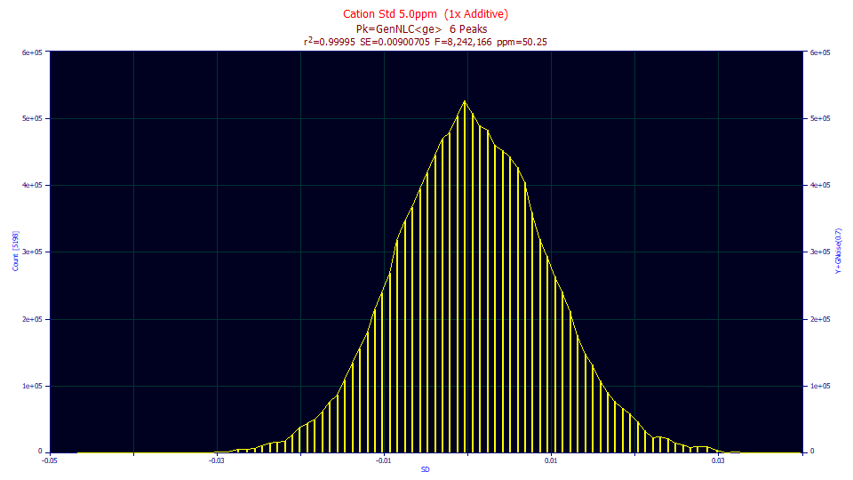
The histogram was formed in this example from over 11,000 residuals. Given the count of data, we would expect the density to look a bit more Gaussian. We cannot say that the residuals aren't normally distributed, merely that they may be suspect.

PeakLab requires at least 16 active data points in order to produce a residuals distribution. Note that any histogram is of dubious merit when data table sizes are small because of the large bin spacing. The greater the number of data points, the more accurate the distribution will be.

Delta Stabilized Normal Probability Plot

PeakLab has historically used this approach as the best way to test that errors are normally distributed. A stabilized normal probability (SNP) plot uses an arctangent transformation on both X and Y to produce a normal probability plot that uses a linear scale for both the X and Y axes. On such a plot, perfectly normal errors plot as a 45 degree line. Critical limits also have a 45 degree slope, and lay equally above and below this line.

PeakLab modifies the SNP slightly and uses a delta SNP, where the X value is subtracted from the Y. This produces a horizontal y=0 for pure normal data, and horizontal critical limit lines.

PeakLab plots 90, 95, 99, and 99.9% critical limit lines on the SNP plot. By default, the 90% lines will be blue, the 95% green, the 99% yellow, and the 99.9% red.

A critical limit for a 10,000 point data set is generated as follows. A million different 10,000 data point sets of normally distributed random values are generated and 1 million SNP curves are computed, and for each the minimum and maximum value are saved. Those are then saved, sorted, and 90, 95, 99, and 99.9 percentile values computed.

A 99% critical limit for a 10,000 point data set means that in only 1 out of 100 such data sets should even a single SNP point violate this limit. You may find the 99% critical limit the most useful. If even a single data point in the SNP violates this 99% limit, it is reasonable to assume that the errors fail this normality test.

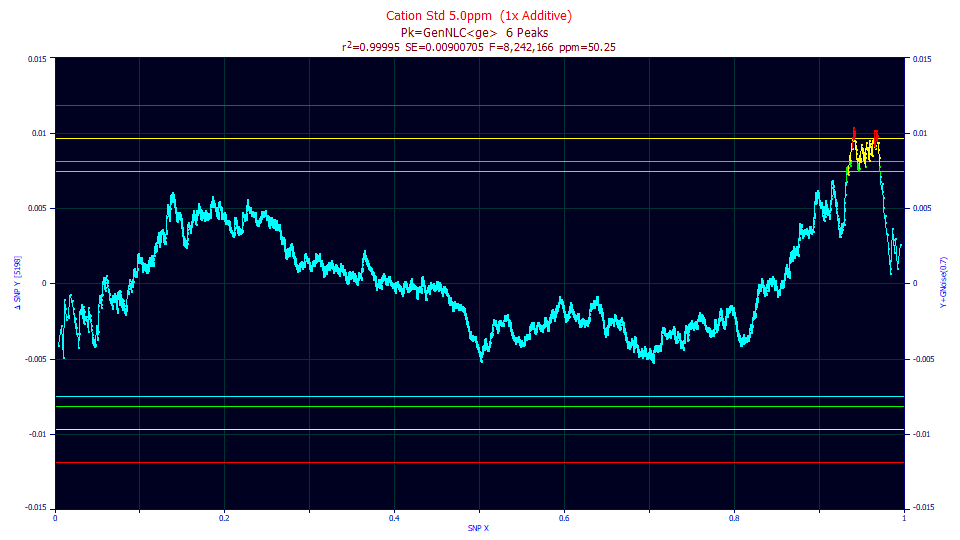
In this example, most of the SNP curve is within bounds, but there are values that violate the 99% upper bound (yellow). These plot as red points.

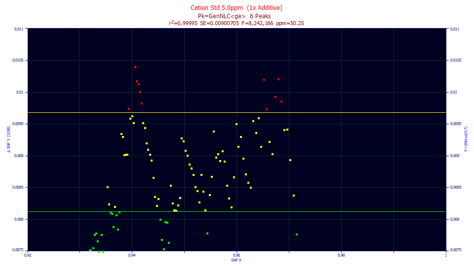
In data sets of this same exact size, containing Gaussian deviates, one SNP point in 100 data sets touched this yellow upper bound. Here, in just one data set, eleven points did so. Using the SNP test as a rigorous standard, you should not report the parameter confidence bounds as valid in any publication. In all likelihood, the actual error bands will be somewhat wider.

If you go directly to the Review without fitting the data, you should always inspect the SNP before attempting to use the parameter confidence statistics in any way. It is altogether likely that the errors present in such a case will be non-normal.

For more information on the SNP, you may refer to:

John R. Michael, "The Stabilized Probability Plot", Biometrika, 70,1, p11-17, 1983.

Lloyd S. Nelson, "A Stabilized Normal Probability Plotting Technique", Journal of Quality Technology, 21,3, 1989.

Parameter Confidence with PeakLab Fits of High Quality Chromatographic Data

In the above fit example example, we see data which slightly failed the Gaussian (normality) tests for residuals.

In our experience, with the high S/N of modern chromatographic data, and with a highly accurate fit where the residuals will be exceedingly small in magnitude, the SNP test will seldom confirm normality. In fact, the better the fit, the greater the likelihood of a small systematic trend existing in what tiny measure of error is left over. In most instances of an excellent fit, you are not likely to be in a position to report as trustworthy the confidence bounds given for the parameters of fit. They are also likely to be so exceptionally narrow that you would have a hard time finding an experienced statistician that would trust such tiny estimates of error.

The systematic trends in the tiny leftover of residuals may be due to the inadequacy of the model to capture the last measure of variance. They may also arise from imperfect baseline subtraction and deconvolution prior to fitting.

This is the non-parametric baseline subtraction for a data set that has an exceptionally high S/N:

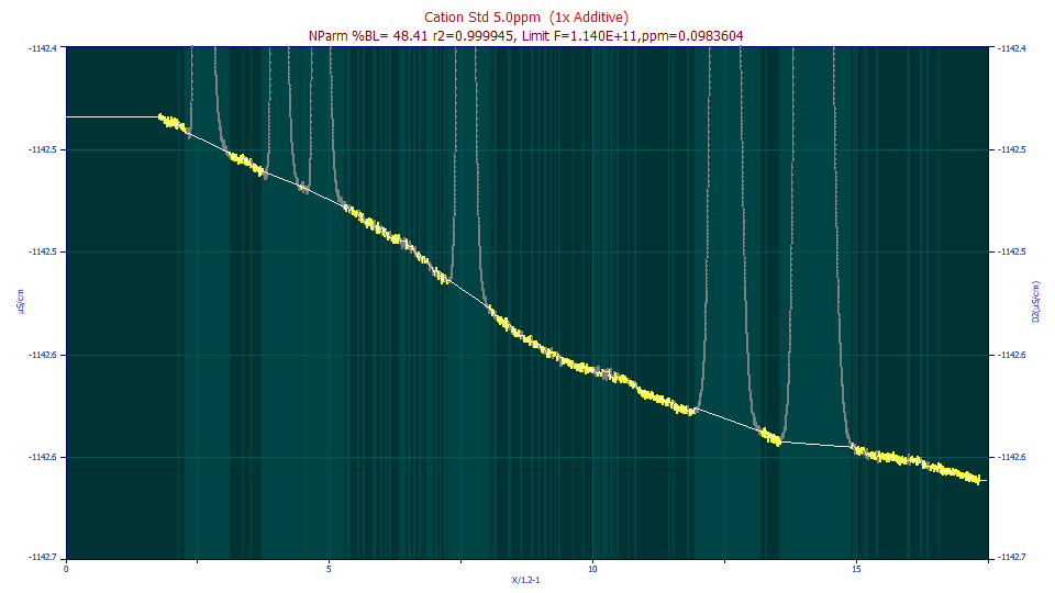
Note the less than perfect trace of the baseline using the non-parametric algorithm.

This is its <ge> IRF deconvolution:

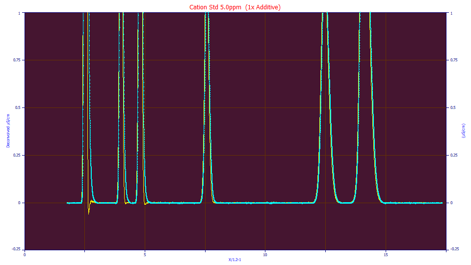
Note the less than perfect deconvolution where the first peak's DC drops slightly below the zero of the baseline.

There are examples of introducing systematic trends in the residuals. There will also be that which the model itself cannot capture, which at especially tiny magnitudes is almost certain to consist of systematic effects.

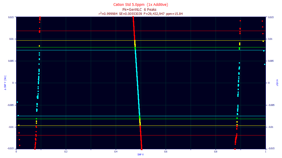
This is the SNP from fitting the above baseline corrected and deconvolved data prior to fitting. The fit is still excellent, 15.8 ppm unaccounted variance. The test for normality, however fails badly, half the SNP points on the other side of the 99.9% bound. One point each in 1000 data sets of this size would be expected to touch the red bounds. Here we have greater count of over 11,000 data points doing violating such a bound.

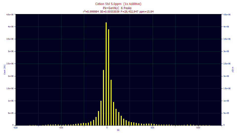
The density looks nowhere Gaussian, fat tails, almost a double sided exponential or Laplace density.

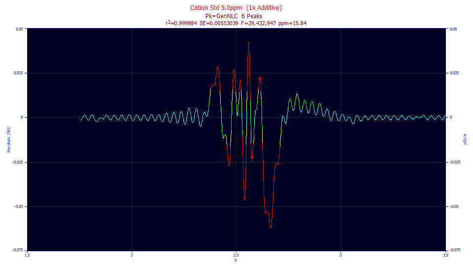
These are the actual residuals, zoomed in to see just the first peak, and plotting these residuals with connected lines. The small systematic oscillations are from the deconvolution and its Fourier domain filter. This is a lovely example of systematic trends and residuals that are not independently and identically distributed (IID), the main requirements for placing one's trust in the least-squares confidence statistics.

Fitted Parameters

r² Coef Det        DF Adj r²          Fit Std Err        F-value            ppm uVar

0.99998416         0.99998413         0.00553039         29,432,947         15.8351778

Parameter Statistics

Peak 1 GenNLC

 Parameter           Value             Std Error         t-value           99% Conf Lo        99% Conf Hi

         Area        1.87021951        9.7887e-5         19105.8095        1.86996732         1.87047169

       Center        2.48808847        1.7474e-5         1.4239e+5         2.48804345         2.48813348

        Width        0.00024350        1.5553e-7         1565.55738        0.00024309         0.00024390

     Distortn        -0.0023604        6.8925e-7         -3424.6814        -0.0023622         -0.0023587

      NLCasym        1.05238967        0.01004548        104.762464        1.02650980         1.07826954

If we look at the parameter statistics for this fit, each parameter is significant. For any respectably sized chromatographic data set, the Student's t for 95% significance occurs at |t|=1.96, and 99% significance occurs at |t|=2.58. Even if the percentage points for the actual non-normal densities were twice these values, the the lowest |t| for peak 1 in this fit (the a₄), is around 105. The parameters are easily seen as significant. The issue rests with the 99% confidence limits about the parameters. With the normality and IID assumption of the residuals violated, we cannot assume the true values rest between the confidence limits assumed with the Student's t density (essentially a normal at the degrees of freedom of a typical chromatographic data set).

The true confidence bands about the parameters will thus be wider than reported here.

While there are computationally intensive bootstrap methods that can get to these actual errors, in the course of our development work with PeakLab's models, with respect to gauging the significance of the parameters in those models, we used the 99% confidence levels as thresholds for significance instead of the 90 or 95% confidence levels. We mostly wanted to see where models were overspecified, where a given parameter was not making a significant contribution to the overall model fit.

We tended not to worry about the normality and confidence when goodness of fits were 50 ppm unaccounted variance (r²=0.99995) and lower, since nearly everything was fitted, and we knew we weren't going to see normality in the tiny magnitude residuals no matter what we did. When fits were that strong, the confidence band of the parameters was exceptionally small, at least in comparison with historical chromatographic modeling.

Maximum Likelihood

When the normal assumption is invalidated due to appreciable tails in the residuals distribution, equally invalidated is the assumption that least-squares is furnishing the maximum likelihood fit. In such a case, one of PeakLab's robust minimizations may represent a better maximum likelihood model. If you choose to fit a robust model, please remember that PeakLab's goodness of fit statistics are all based on a least-squares common frame of reference. As such, the goodness of fit values will fail to reflect the improvement derived from switching to a robust method. One of the key reasons for using a robust method in the past was to realize a higher dynamic range on the Y-variable, more effectively fitting small amplitude peaks in the presence of much larger ones. This had made a difference even with baseline resolved peaks. In PeakLab's advanced fitting strategies, you should not have to resort to a robust minimization to successfully fit peaks with a broad range of areas.