PeakLab v1 Documentation Contents            AIST Software Home            AIST Software Support

PeakLab Review

The PeakLab Review is available at the conclusion of Graphical Fitting, and from the three AutoFit (automated fitting) options. It is available whether or not the data have been fitted, although cautions are in order when reviewing unfitted data.

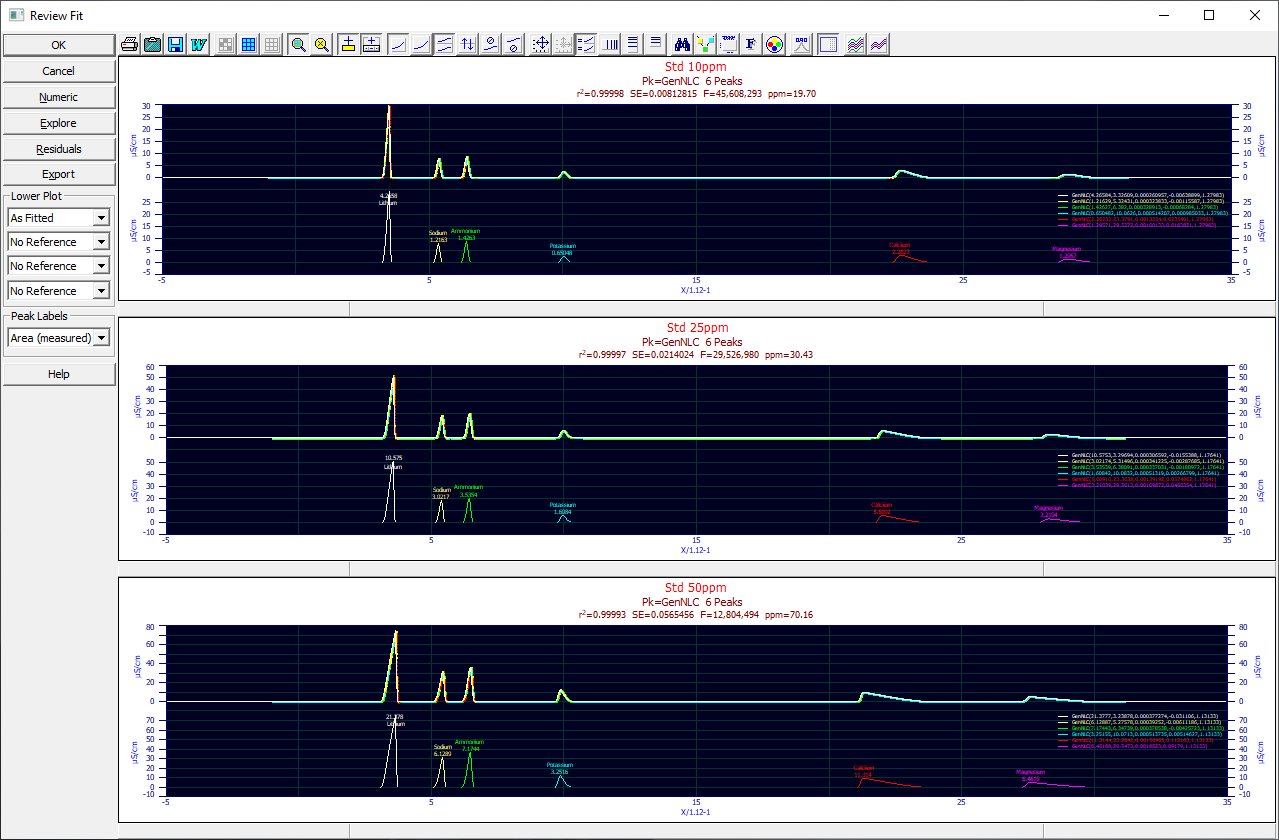
The Review consists of a PeakLab Graph containing both a Y and Y2 plot. The component peak functions are shown in the Y-axis plot. The Y2 plot contains the fitted curve, the data that was fitted, and the baseline, if one was included in the fit. By default, the data points are colored by relation to the fit standard error.

Selective Review

When multiple data sets are fitted, all are shown in the Review.

If you wish to compare only certain fits, select those you wish to review by clicking on the specific graph for that fit (the border will turn gray to indicate selection). You can also use the Select this Graph right click menu option for each fit. You can click again on a selected set to deselect it, or use Unselect this Graph from the right click popup menu. When the sets you wish to individually review are selected, select the Plot | Only Selected Fits from the right click menu. Only those data fits will be rendered in the Review graphs, in the Numeric Summary, in the Residuals, in the Explore option, and in the Export.

If you only wish to review one of the fits, you can double click that graph to open a review of just that fit. You can also choose Plot this Fit (or Plot Only this Fit) from the right click menu. When you are finished, and you wish to restore all of the fits, you can once more double click the graph or select Plot All Fits.

Review Graph

Peak Labels

The Review graph's toolbar offers the means to add Peak Labels to the graphs. These include parameters, moments, and measured properties from the fitted peaks. The Peak Labels are also available in the Peak Labels dropdown in the dialog.

Data Titles Legend

The Show or Hide Legend Titles toolbar option will display or hide the titles for the different data sets. The titles are first placed to left of the plot. Clicking this item again will place the titles to the right. Clicking yet again will toggle the titles off.

Confidence Intervals

The Review graph offers the option of displaying Confidence and Prediction Intervals about the fitted curve.

The Set Confidence/Prediction Intervals, % Confidence button is used to set confidence interval type and percentage. The option opens a simple dialog where you can individually check Confidence Intervals and Prediction Intervals, and where you can select from 90% Confidence, 95% Confidence, and 99% Confidence.

The Show Confidence/Prediction Intervals button toggles the currently set intervals on and off.

The selected confidence level applies not only to the confidence and prediction intervals in the graph, but also to confidence limits on the parameters in the Numeric Summary, and to the confidence and prediction ranges for the data in the Data Summary.

Lower Plot

There are four dropdowns. You can render a peak in up to four different representations. The additional renderings, by default, follow a R-G-B (red-green-blue) color scheme. These are the AuxComp1, AuxComp2, and AuxComp3 colors which you can change in the Custom Colors option. For each of the four renderings you can choose:

As Fitted

This is the peak exactly as given by the fitted model. These are the peaks you actually see from the instrument.

No Reference

This is available for all except the first dropdown. Nothing is rendered.

IRF Deconv.

This the the peak absent the IRF. You must fit an <irf> bearing model for this option to plot a peak with this instrument response function removed. For a GenNLC<ge> model, this option will display the GenNLC model with no <ge> IRF distortion. This deconvolution comes directly from fitting an <irf> model. These are the peaks you would see with a perfect instrument/system that introduced zero distortion.

For spectroscopy data, the Gaussian and Lorentzian components of a Voigt peak are shown using the Partial Deconv. and Full Deconv. selections.

Partial Deconv.

This the the peak absent both the IRF (instrument response function) and the ZDD deviation (from the expected theoretical zero distortion density). This is generally used to see pure the pure HVL peaks when you have fit a GenHVL model, or pure NLC peaks when you have fit a GenNLC model. The ZDD deviations from the theoretical expectation are discarded in this deconvolution which comes directly from fitting one of the models in the GenHVL or GenNLC families. These are the peaks you would see at current concentrations if the HVL diffusion or NLC kinetic assumptions were perfect and registered by a perfect instrument/system that introduced no distortion.

Full Deconv.

This the the peak absent the IRF (instrument response function), the ZDD deviation (from the expected theoretical zero distortion density), and also absent the a₃ chromatographic distortion arising from concentration. This is generally used to see pure the pure Gaussian peaks when you have fit a GenHVL model, or pure Giddings peaks when you have fit a GenNLC model. The chromatographic distortions are discarded in this deconvolution which comes once again from directly from fitting one of the models in the GenHVL or GenNLC families. These are the peaks you would see at infinite dilution if the HVL diffusion or NLC kinetic assumptions were perfect and registered by a perfect instrument/system that introduced no distortion.

State-1

For the experimental two-component ZDD models, you can display the state 1 component. For the GenHVL[Z|E] this is the primary component arising from the 'Z', the generalized normal in the ZDD.

State-2

For the experimental two-component ZDD models, you can display the state 2 component. For the GenHVL[Z|E] this is the secondary component arising from the addition of the 'E', the EMG in the ZDD.

Deconvolution Display Examples

Chromatographic Peaks

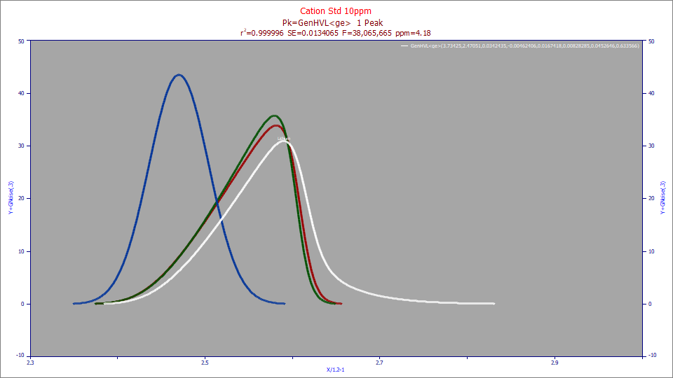
For chromatography convolution models with an <irf> instrument response function, and all other models that include an IRF, the IRF Deconv. option will display the peak with these instrumental distortions removed. For the chromatographic peak in the above plot, the white curve is the observed peak and the red curve contains the peak with the IRF removed. The green curve shown above appears when selecting the Partial Deconv. option. This will be the pure HVL peak in a generalized HVL model and the pure NLC peak in a generalized NLC model. The blue curve shown above appears with the the Full Deconv. selection. For generalized HVL models, this will be a Gaussian peak, and for the generalized NLC models this will be a Giddings peak, essentially what the peak would look like in the approach to infinite dilution.

Spectral Peaks

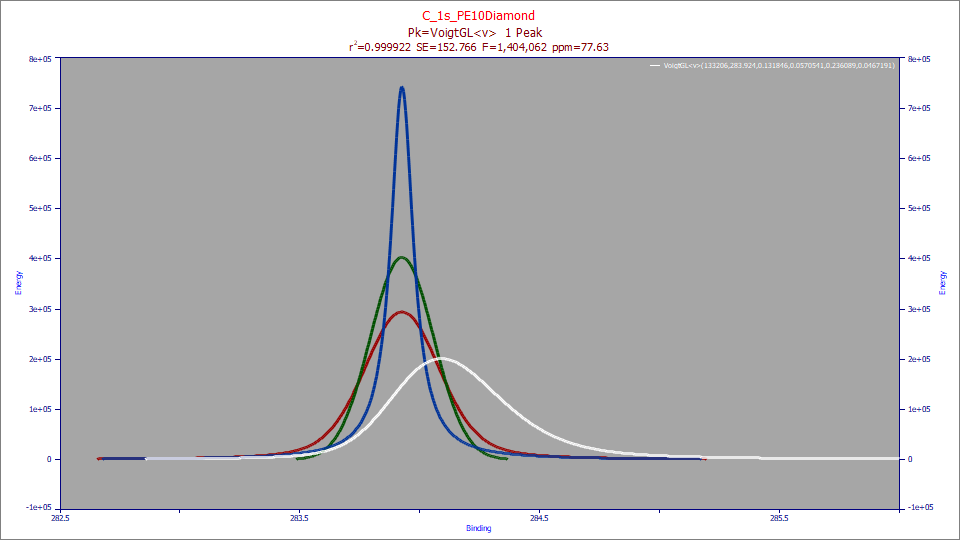
For spectroscopy, the Voigt is treated as a 2-component convolution instead of the convolution of a Gaussian IRF with a primary Lorentzian peak. Unless you fit an <irf> convolution model with the Voigt, you will only see the original data in the IRF Deconv. setting. In the above example, we fit a Voigt model with a <v> one-sided Voigt IRF to an asymmetric X-ray spectral peak where the primary peak is a full Voigt. The white is the peak as observed by the instrument. The red curve is the peak with this directional one-sided Voigt IRF removed. In a Voigt<irf>, all of the deconvolutions will be symmetric and based on the primary Voigt peak. The green curve is the Gaussian component of the primary Voigt which is deconvolved in the fitting, and is shown with the Partial Deconv. selection. The blue curve is the deconvolved Lorentzian within the Voigt, and is displayed with the Full Deconv. option.

Peak Labels

You can use the Peak Labels dropdown instead of the Peak Labels option in the toolbar of the graph.

Numeric

The Numeric button is used to display a full Numeric Peak Analysis for all data sets. To see the numeric summary for an individual data set, right click the data of interest and select View Numeric Summary for this Fit from the popup menu. The Numeric Summary a live window that can remain up while different data sets are selected or deselected for review. The Numeric Summary will be automatically updated.

Explore

The Explore button opens a set of PeakLab Graphs which furnish an extensive graphical exploration of parameter and property relationships in the fits. In experiments, you can assign your own experimental process variables to the different data sets which are then optionally used in this Explore feature. The Explore window is also live and can remain up while different data sets are selected or deselected for review. The Explore view will be automatically updated. You should use the right click menu option Map Experimental Process Variables to specify up to four process variables for each experiment in a matrix of data sets. Once specified these are then available for the graphs in the Explore option and automatically saved in the PeakLab data file.

Residuals

The Residuals button opens a PeakLab Graph containing the residuals from the peak fit. The residuals are the difference between the data and fitted curve. If you have entered the Review without first fitting the data, you should inspect an SNP plot to test the normal assumption of errors before attempting to use any of the standard error or confidence limit statistics. The Review window is also live and can remain up while different data sets are selected or deselected for review. The Review view will be automatically updated.

Export

The Export option is used to write the Numeric Summary or a Data Summary or both, for all of the data sets fitted, to an ASCII file.

Right Click Menu Options

Many of the options you may find important in the Review are only available from a right click popup menu, and many will pertain to just a single fit. When you right click a graph, a popup menu will offer the following options:

Restore Scaling - Undo Zoom

If you have zoomed in the graphs, this option can be used to undo the zoom-in and restore the automatic scaling.

Select this Graph

Use this right-click menu option to select a specific data set. This is used for reviewing/comparing only certain data sets and excluding others. A selected fit's graph will be bounded with a gray rectangle. You can also select a fit by left clicking its graph. When the sets you wish to individually review are selected, select the Plot | Only Selected Fits from the right click menu. Only those data fits will be rendered in the Review graphs, in the Numeric Summary, in the Residuals, in the Explore option, and in the Export option.

Unselect this Graph

Use this right-click menu option to unselect a selected data set. The highlight of the bounded gray rectangle is cleared. You can also unselect a selected fit by left clicking its graph.

Plot this Fit, Plot | Only this Fit

If you only wish to review one of the fits, you can double click that graph to open a review of just that fit. You can also choose Plot this Fit (or Plot | Only this Fit) from the right click menu. When you are finished, and you wish to restore all of the fits, you can once more double click the graph or select Plot All Fits.

Plot | Only Selected Fits

If you wish to compare only certain fits, select those you wish to review by clicking on the specific graph for that fit (the border will turn gray to indicate selection). You can also use the Select this Graph right click menu option for each fit. You can click again on a selected set to deselect it, or use Unselect this Graph from the right click popup menu. When the sets you wish to individually review are selected, select the Plot | Only Selected Fits from the right click menu. Only those data fits will be rendered in the Review graphs, in the Numeric Summary, in the Residuals, in the Explore option, and in the Export. The Numeric Summary, Residuals, and Explore options are 'live' and will update as you change the fits that are plotted.

Plot All Fits

If you have chosen to plot selected fits, or just a single fit, you can use this right click popup menu option to restore all graphs. If you double clicked a graph to review a single fit, you can double click that individual graph to restore all data plots.

Specify Array Layout for Multiple Graphs...

This option opens a Graph Array Layout dialog where you can specify the default count of graphs arrayed across the rows in the graph display grid for each total count of graphs.

Modify Graph Titles for this Fit

The option opens the custom titles option for this specific graph. There is also a titles option in the graph's toolbar which cycles through the graphs for all data sets.

View Numeric Summary for this Fit

This option opens the Numeric Summary with only the content for the specific fit where this right click popup was invoked. If the window is already open, it is updated with just this specific fit.

Close Numeric Summary

This option closes the Numeric Summary window. You can also close this window directly or click the Numeric button.

AIA Import File Information for this Data Set

This option displays the AIA source information if the data originated from an AIA net CDF data file.

View Data Summary for this Fit

This option opens a Data Summary containing a window listing the residuals of fit and the estimations and confidence and prediction limits on a point by point basis.

Evaluate Fit Model

This option opens the Evaluation feature where you can directly compute function, derivative and cumulative estimates, and generate tables based on the fit. This option is only available from the right click popup and will only apply to the fit in the graph where this right click was made to open the popup menu.

View Residuals Graph for this Fit

This option opens the Residuals with only the data for the specific fit where this right click popup was invoked. If the Residuals window is already open, it is updated with just this specific residuals graph.

Export this Fit to ASCII File

This option opens the Export dialog and writes the Numeric Summary or a Data Summary or both, but only for the fit in the graph where this right click was made to open the popup menu.

Export this Fit to Windows-style INF File

If you wish to programmatically extract ASCII information from an exported fit file, this may be helpful. This uses the Windows INF type of ASCII file to store the fit information. The format is self-explanatory.

Export this Fit to Extended AIA netCDF File

If you have implemented a netCDF program for moving data to and from your own applications, you may find this option useful. All of the PeakLab information is stored in variables that begin with pkfit_. None of the variables violate the names specified in the chromatography standard. If the data originated with an AIA file, that information will also be copied to the new file.

Map Identifying Labels to Specific Peaks

This option opens a Map Identification to Peaks dialog where you can specify labels to assign to peaks based on either position in the fit or x range.

Map Experimental Process Variables for Fitted Data Sets

This option opens a Map Experimental Process Variables dialog where you can specify up to four process variables for each experiment in a matrix of data sets. These are then available for the graphs in the Explore option.

Explore Parameters and Properties for Fitted Data Sets

This right click menu option opens the Explore option for all data sets. You can also use the Explore button in the dialog. This opens a set of PeakLab Graphs which furnish an extensive graphical exploration of parameter and property relationships in the fits. If you have assigned experimental process variables to the different data sets, these will be available in the Explore feature.