PeakLab v1 Documentation Contents            AIST Software Home            AIST Software Support

Explore

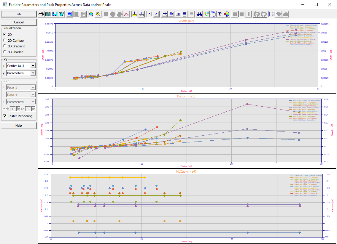
This Explore option in PeakLab's Review is used to graphically explore the relationships between parameters, properties, moments, fit statistics including experimental process variables you have identified as part of the data sets fitted. The Explore window is live and can remain up while different data sets are selected or deselected in the Review.

The dialog is used to specify the graphs you wish to see as well as the type of graph to be rendered.

Visualization

There are four options:

· 2D - an X,Y plot is rendered

· 2D Contour - an X,Y,Z plot is rendered, Z in a contour (as a surface would be seen from above, with a 90 degree view angle)

· 3D Gradient - an X,Y,Z plot is rendered, the surface rendered as a gradient plot (Z color gradients)

· 3D Shaded- an X,Y,Z plot is rendered, the surface rendered as a shaded plot (illumination or reflected light)

XY

This will be the only option if insufficient data exists for a 3D plot.

x

· Peak # - the peak number in sequence

· Data # - the data set number in sequence

· Center (a1) - the a1 parameter value of each peak

· Center (mode) - the apex value of each peak

· Area (a0) - the area parameter of each peak

· Width (a2) - the width parameter of each peak

· Distortion (a3) - the distortion parameter of each peak

If you have assigned process variables to the fits, these are included in the x list.

y

· Parameters - all parameters in the fitted peak model a0, a1, a2, etc.

· Properties - Amplitude, Center, FWHM, Asym50, FW Base, Asym10

· Moments - Area, Mean, StdDev, Skew, Kurtosis

· Fit Statistics - ppm, r2, SE, Fstat

· Props/Moments - Properties and Moments as above

· Parms/Props - Parameters and Properties as above

· Parms/Moments - Parameters and Moments as above

XYZ

This will be available only if sufficient data exists for a 3D plot.

x,y

· Peak # - the peak number in sequence

· Data # - the data set number in sequence

· Center (a1) - the a1 parameter value of each peak

· Center (mode) - the apex value of each peak

· Area (a0) - the area parameter of each peak

· Width (a2) - the width parameter of each peak

· Distortion (a3) - the distortion parameter of each peak

If you have assigned process variables to the fits, these are included in the x and y lists.

z

· Parameters - all parameters in the fitted peak model a0, a1, a2, etc.

· Properties - Amplitude, Center, FWHM, Asym50, FW Base, Asym10

· Moments - Area, Mean, StdDev, Skew, Kurtosis

· Fit Statistics - ppm, r2, SE, Fstat

· Props/Moments - Properties and Moments as above

· Parms/Props - Parameters and Properties as above

· Parms/Moments - Parameters and Moments as above

Peak

For many options, the 25 graph limit will be exceeded. Use the Peak dropdowns to set a narrower range of peaks. To see a single peak 3, assuming peak 3 is the same solute across all of the fits, enter 3 in both of the dropdowns.

Faster Rendering

For 3D plots, this option will automatically adjust the 3D settings to speed up rendering. This allows the full resolution graphs to be available in the various output options without having to make any modifications. The Faster Rendering option forces a 60x60 grid in both contours and 3D surfaces. When Faster Rendering is off, the graphs will display at full resolution. The Faster Rendering also disables the mesh Trace and uses a low resolution in the spectral gradients.

Selective Viewing

Data Sets/Fits

These are selected in the main Review graphs window (the Explore graphs are simultaneously displayed with these main Review graphs). Select the data sets/fits you wish to have in the explore function by clicking the various main Review graphs to highlight them with the gray border (or right clicking and choosing Select this Graph). Choose Plot | Only Selected Fits from any graph in the main Review window to plot a subset of the data sets/fits. These will be reflected in the Explore graphs. Note that the a 3D graph may be converted to 2D if the information necessary for a 3D rendering is no longer sufficient.

Explore Graphs

These are selected in the Explore graphs window. Select the Explore graphs you wish to selectively view by clicking the various Explore graphs to highlight them with the gray border (or right clicking and choosing Select this Graph). Choose Plot | Only Selected Graphs from any graph in the Explore window to plot a subset of the Explore graphs.

Specific Peaks

For 3D plots, select the peak of interest in both dropdowns, or specify a contiguous range. To see the graphs for peaks 2 through 4, specify 2 in the first Peak dropdown and 4 in the second.

Animation

The gradient and shaded surfaces can be rotated (animated) in real time to view the surface at a succession of X and or Y viewing angles.

Use the Modify 3D Animation Settings toolbar button to set the angles and increments for the animation.

Use the Start/Stop 3D Animation toolbar button to begin and end the animation. You can temporarily pause the rotation by left clicking the graph. Clicking again will continue the animation.

Use the Modify Graph View toolbar button to change the main 3D settings.

Use the Select Color Gradient for Surface or Contour toolbar button to change the gradient used in the 3D surface plots.

Use the Render 3D Surfaces with Plateau at Upper Z Bound to have the upper Z-bound filled rather than open.

The Animation settings include a maximum grid setting to improve performance during animation.

The Faster Rendering option forces a 60x60 grid in both contours and 3D surfaces. Unless you set a lower maximum grid in the animation the Faster Rendering settings will prevail. If Faster Rendering is unchecked, the animation will proceed at no higher density than the maximum grid in the Animation settings, whose default is 120x120. If you uncheck Faster Rendering, the animation may be significantly slower, the surfaces of a higher resolution.

Wheel Button Mouse Rotation

If you have a mouse with a middle button wheel, you can change 3D view angles using this wheel button. You can do this from the Explore window when 3D graphs are being rendered.

To rotate the surface by XY angle, rotate the wheel upwards to increase the XY angle, downwards to decrease the XY angle. The rotation will be in 5 degree increments. If you hold the Ctrl button down while rotating the wheel the XY rotation will be in 10 degree increments.

To rotate the surface by Z angle, hold the Shift key down and rotate the wheel upwards to increase the Z angle, downwards to decrease the Z angle. The rotation will be in 5 degree increments. If you hold the Ctrl button down while rotating the wheel the Z rotation will be in 10 degree increments.

If your wheel mouse has a tilt wheel, you can also increase the Z angle toward +90 degrees by holding the tilt button to the right and releasing it when you have the angle you wish. You can decrease the Z angle toward -90 degrees by holding the tilt button to the left until the desired angle is rendered. The rotation will be in 5 degree increments. If you hold the Ctrl button down while holding the tilt wheel left or right, the Z rotation will be in 10 degree increments.

When multiple graphs are present, the first graph is rotated and the others asynchronously adopt the same angles. You may need to pause for a few seconds to allow all of the graphs to catch up. When using the mouse, the first graph will always reflect the state of the angles and you should look at that one to affirm the view you wish to use. Certain of the other graphs may not catch up until the mouse adjustments are completely finished. In PeakLab, all 3D graphs in a multiple graph procedure share the same view.

Understanding 3D Rendering

When you enter your own process variables, there will be just one x and y for each peak and each parameter or property you are viewing. This will mean surfaces are often being rendered across large zones of xy space where no data exists. This is an important point since you want to be certain you are looking at the true picture of the experimental relationships and not an artifact of the rendering. By default, the 3D rendering will consist of a C1 (one continuously differentiable) interpolant (there is no smoothing-each point passes directly through the surface). This is fine when there is a clearly defined surface.

Clearly Defined Planar Surface

For this case, will use the often lovely a₃ distortion relationships you will see as a function of sample concentration and many other variables which impact the distortion (intrinsic tailing or fronting) in the GenNLC and GenHVL models. Here we show both the Contour and 3D Gradient in succession for a peak that is very close to the transition between fronting (-a₃) and tailing (+a₃) for experimental variations in concentration and additive level.

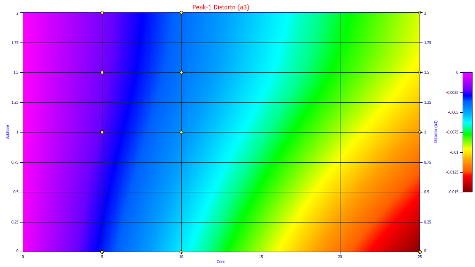
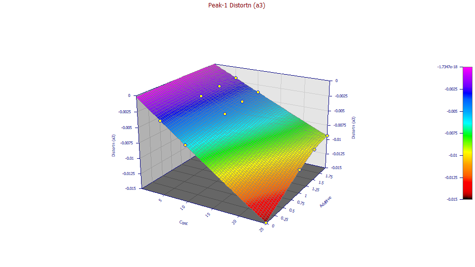
Here we can ignore the autoscaled concentration below 5ppm where no data exists. The a₃ trend with concentration trend is obvious, but there is also a clear a₃ trend with additive level at each of the three sampled concentrations. The distortion becomes more positive with increasing additive (the fronted peak becomes less fronted). The contour will offer more detail, but only from this view of looking straight down from above at the surface. The contour depends entirely on coloring where the gradient and shaded plots render a picture of the surface in 3D space. In this data set, because the surface is planar, the shaded surface will offer little visualization value. There are no features in the surface that are highlighted or shadowed.

Non-Planar Surfaces

Here we will look at a₅, the Gaussian component in the <ge> IRF. This will be identical for all peaks since the IRF parameters are shared. Here we do want to see the 5-25 scale on the x-axis. From the contour plot we will zoom the data so that only 5-25 is shown on the x-axis:

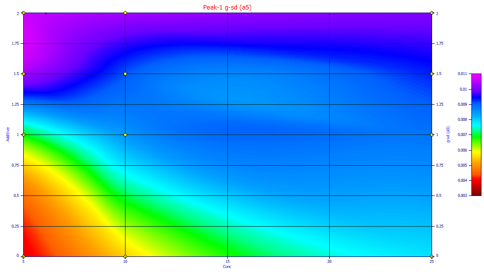
Here we see the reverse. The concentration impacts the 'g' component of <ge> IRF, but the additive level appears to have the stronger influence. When the contour is zoomed 5-25, that scale automatically carries over to the gradient and shaded plots.

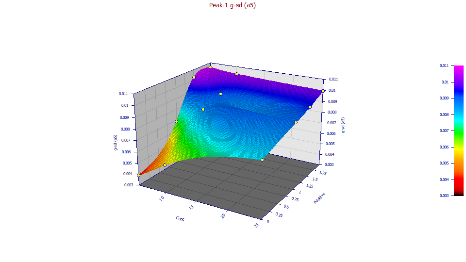
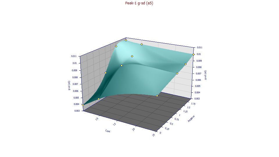
At low sample concentrations, the additive effect significantly increases the half-Gaussian in the IRF. This could be for any number of reasons. We would start with the assumption that this component of the IRF may possibly be related to axial dispersion in the system. Although these surfaces are enough to discern the trend, you will often want to refine the 3D rendering to remove all anomalies arising from noise in the data.

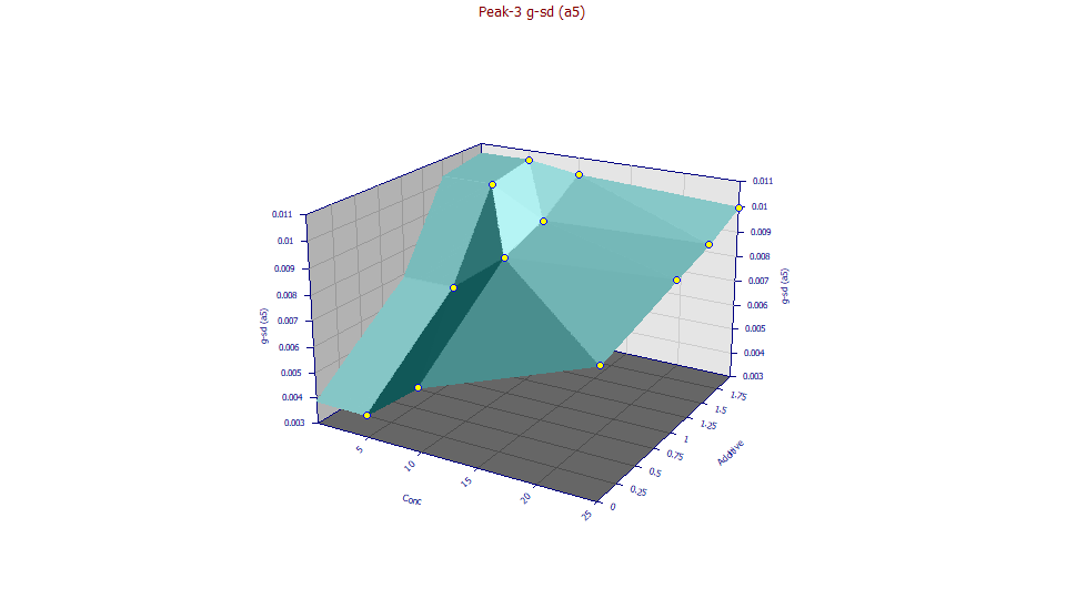
C0 Interpolant

When the data are sparse and the C1 (continuous and smooth) interpolant introduces undulations in the surface, you can use the Specify Surface Modeling toolbar button to select a C0 (continuous, but not smooth) interpolant. The C0 surface will create triangular planes between the points allowing the lack of smoothness in the surface to be seen. The shaded surface is especially useful for this visualization.

Smoothing

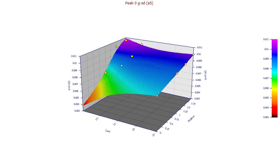
You can also create a 3D Loess smoothed surface. In the following, Loess smoothed data is used with a C1 interpolant passing through the smoothed points (the Fast Smooth option). Here you want to use the lowest level of smoothing that gives you a smooth surface free of artifacts. Here we use a model order 2 (quadratic) for the Loess smoothing and a 12 nearest neighbor count (all of the points in the surface). The smoothing allows the trends to be more clearly observed. On especially noisy data sets, you may need to use very high smoothing levels.

Use the interactive adjustments in the Specify Surface Modeling option liberally to ensure all rendered surfaces, and inferred trends, are valid.