PeakLab v2 Documentation Contents R2N Software Home R2N Software Support
Segment Fit
Segment-Based Placement
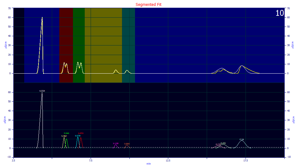
Each of the three peak fitting options offer the Use Baseline Segments option. This will be available when a baseline has been subtracted in a preprocessing step. In a segment placement, the peaks resting between baseline segments are treated as separate sectioned data sets.

Each segment that was identified by the baseline processing will be displayed with a different background color. There may be any number of peaks within a given segment, including just a single baseline-resolved peak. In the above example, the baseline processing identified six segments. The ten placed peaks are partitioned into these six segments, the last segment with three peaks.
When the Use Baseline Segments box is checked, the starting estimate algorithms will treat each of the segments as a separate data set, adjusting widths based on the areas of the peaks within each particular segment.
This segment-based placement doesn't mean that a segmented fit will automatically occur in any subsequent fit. This Use Baseline Segments setting affects only the placement of the peaks, but it also furnishes a visualization of the identified baseline segments which will be used in a segmented fit, should you choose to have this take place.
Segment-Based Fitting
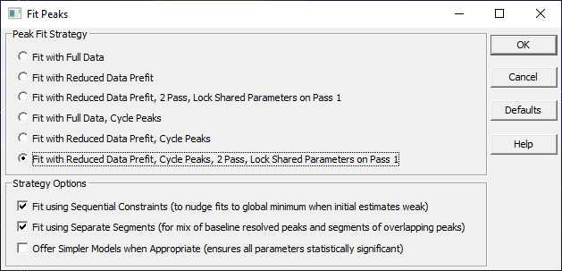
To perform a fit where each segment is treated as a separate data set, you must check the Fit using Separate Segments (for mix of baseline resolved peaks and segments of overlapping peaks) box in the dialog that precedes the fitting:
One of the key concepts in a segment fit is that a segment with multiple peaks will contain peaks with some measure of overlap, peaks that will not be baseline resolved. The assumption in a segment fit is that there may not be enough information in the overlapping peaks to accurately fit independent a2 widths and a3 distortions with any accuracy. Such is a perfectly valid assumption. The greater the measure of overlap, the less the information in the segment will support the fitting of separate a2 widths and a3 distortions for the overlapping peaks.
In a segment fit, each segment will be fitted as if it were a separate data set. This means the Vary width a2 and shape a3 boxes apply only intra-segment. If these boxes are unchecked, all of the peaks within that segment will share the same a2 width and a3 distortion. Each segment will be addressed separately. The next segment, if also containing multiple peaks, will likewise fit a shared a2 width and a3 distortion, but these values will bear no relation to those in any other segment. The a2 widths and a3 distortions will thus vary across segments, but not within them.
In general, you will uncheck the width a2 and shape a3 boxes in the Vary section of the placement dialog in order to have the overlapping peaks in each segment fitted with a shared a2 width and a3 distortion.
Automatic Segment Determination
The segments are automatically determined by the baseline subtraction level nearest the current data level. It is possible to have more than one baseline subtraction. Such may be necessary if it is apparent that the shared a2 and a3 assumption within a segment does not hold across all of the segments. In this example, the three peaks in the last segment are hardly placed with the same accuracy as those within the second and third segments.
When the Use Baseline Segments box is checked, the starting estimates will honor the width a2 and shape a3 states as if one will proceed with a segment-based fit. These are the values shown in the fitting procedure's List option:
Peak Type a0 a1 a2 a3 a4
1 GenNLC 11.1290488 4.12464408 0.00025337 -0.0099189 1.18580000
2 GenNLC 1.63867012 5.80121665 0.00026275 0.00031198 1.18580000
3 GenNLC 1.44295428 5.95856407 0.00026275 0.00031198 1.18580000
4 GenNLC 1.83041795 6.68948747 0.00026595 0.00031577 1.18580000
5 GenNLC 1.74669467 6.88577555 0.00026595 0.00031577 1.18580000
6 GenNLC 0.80828824 9.17430946 0.00036095 0.00127690 1.18580000
7 GenNLC 0.80153386 9.93080502 0.00039563 0.00212049 1.18580000
8 GenNLC 1.50052900 15.7895325 0.00134629 0.00159850 1.18580000
9 GenNLC 2.33426611 16.1071172 0.00134629 0.00159850 1.18580000
10 GenNLC 4.54387311 17.2942595 0.00134629 0.00159850 1.18580000
Visually inspecting the raw data, it is clear that the shared width and distortion assumption may be fine for the second and third segments, but not the last. The peaks are too sharply changing width and distortion at the far end of the chromatogram. There needs to be a segment between the two peaks with strong overlap, and the last peak which is almost fully baseline resolved, but which did not identify as such in the baseline processing.
A Second Baseline Preprocessing
We thus perform a second baseline subtraction preprocessing where we ensure a baseline exists between these peaks. For the sake of this example, we will manually set this new baseline so that the sixth and seventh peaks, which were previously detected as separate, are placed in the same baseline segment.
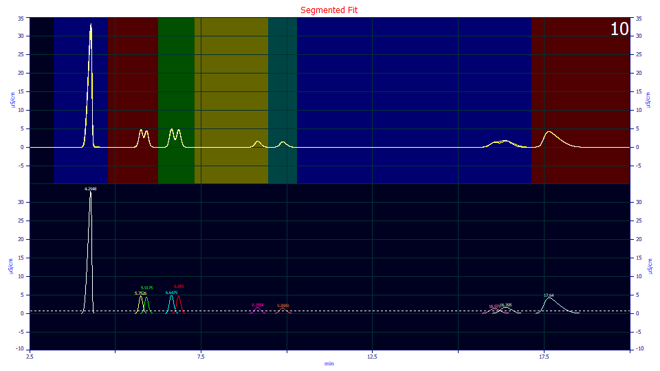
There are now seven baseline resolved segments from this second baseline step. The last peak now has its own segment. The only way to specify different segments is by a new baseline subtraction (this approach enforces baseline-resolved segments rather than allowing them to be arbitrarily specified).
The Non-Segment Fit
We can now fit the data with and without this segmented fit. We do a non-segmented fit by checking the width a2 and shape a3 boxes in the Vary section of the placement dialog and by unchecking the Fit using Separate Segments (for mix of baseline resolved peaks and segments of overlapping peaks) box in the fit strategy dialog:
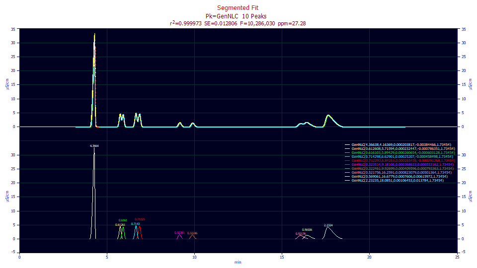
We have a very good fit. For IRF preprocessed data, 27 ppm unaccounted variance and an F-statistic of 10.28 million is excellent. All of the parameters are significant, and apart from only minor deviations, the a2 width increases with retention time. The a3 distortion is completely consistent, fronted to tailed. The a4 ZDD asymmetry is almost always shared across all peaks.
Fitted Parameters
r2 Coef Det DF Adj r2 Fit Std Err F-value ppm uVar
0.99997272 0.99997262 0.01280603 10,286,030 27.2789721
Peak Type a0 a1 a2 a3 a4
1 GenNLC 4.36638259 4.16368695 0.00020382 -0.0038447 1.73454007
2 GenNLC 0.61260761 5.71593860 0.00023245 -0.0007864 1.73454007
3 GenNLC 0.61610261 5.89428834 0.00026065 -0.0006031 1.73454007
4 GenNLC 0.71429836 6.62900942 0.00025207 -0.0004585 1.73454007
5 GenNLC 0.71229305 6.84261002 0.00026548 -0.0002913 1.73454007
6 GenNLC 0.32351443 9.18106091 0.00036863 0.00055316 1.73454007
7 GenNLC 0.32246135 9.92698775 0.00040960 0.00079336 1.73454007
8 GenNLC 0.52175590 16.2591094 0.00082308 0.00501364 1.73454007
9 GenNLC 0.56906077 16.6779205 0.00076060 0.00615972 1.73454007
10 GenNLC 2.23235252 18.0850837 0.00106453 0.01378402 1.73454007
The Segment Fit
In this segment fit, peaks 2 and 3, peaks 4 and 5, and peaks 8 and 9 will share the same a2 width and a3 distortion. For the segmented fit to represent a clear and unambiguous improvement, we need to see all parameters significant, a better F-statistic, and a consistent trend in a2 increasing with retention. We do the segmented fit by unchecking the width a2 and shape a3 boxes in the Vary section of the placement dialog and by checking the Fit using Separate Segments (for mix of baseline resolved peaks and segments of overlapping peaks) box in the fit strategy dialog:
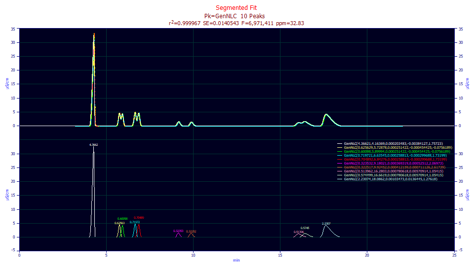
Fitted Parameters
r2 Coef Det DF Adj r2 Fit Std Err F-value ppm uVar
0.99996717 0.99996702 0.01405429 6,971,411 32.8297967
Peak Type a0 a1 a2 a3 a4
1 GenNLC 4.36620829 4.16369126 0.00020348 -0.0038413 1.75723189
2 GenNLC 0.62562905 5.72877712 0.00025142 -0.0004544 -0.0756189
3 GenNLC 0.60098032 5.89993879 0.00025142 -0.0004544 -0.0756189
4 GenNLC 0.71972091 6.63544978 0.00025881 -0.0002997 1.73199288
5 GenNLC 0.70489204 6.84276015 0.00025881 -0.0002997 1.73199288
6 GenNLC 0.32353187 9.18021406 0.00036932 0.00052512 2.06973298
7 GenNLC 0.32251737 9.92452361 0.00041216 0.00071113 2.61738816
8 GenNLC 0.51396194 16.2803260 0.00078062 0.00570914 1.05415262
9 GenNLC 0.57449926 16.6618619 0.00078062 0.00570914 1.05415262
10 GenNLC 2.23073609 18.0861882 0.00103473 0.01364446 1.27617574
Here we see an issue. Since each segment is treated as a separate data set, the a4 asymmetry (deviation from the NLC's ZDD) is fitted separately for each segment. In three of the segments, not surprisingly those with the overlapping peaks, the a4 is insignificant (grayed).
We will thus do one more segment fit. The ZDDs (zero-distortion densities) are often as consistent as the IRFs, at least with a healthy column. The average of the significant a4 values is 1.748. In the non-segmented fit, a4 fit to 1.735. We will use the ZDD option to lock the GenNLC a4 at 1.74, treating this ZDD GenNLC asymmetry as a known constant:
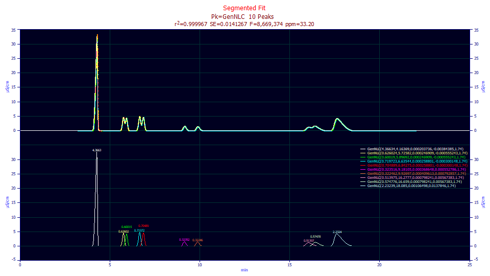
Fitted Parameters
r2 Coef Det DF Adj r2 Fit Std Err F-value ppm uVar
0.99996680 0.99996668 0.01412671 8,669,374 33.1985834
Peak Type a0 a1 a2 a3 a4
1 GenNLC 4.36634064 4.16368798 0.00020374 -0.0038438 1.74000000
2 GenNLC 0.62602443 5.72581829 0.00024691 -0.0005552 1.74000000
3 GenNLC 0.60018991 5.89692287 0.00024691 -0.0005552 1.74000000
4 GenNLC 0.71972261 6.63543589 0.00025880 -0.0003001 1.74000000
5 GenNLC 0.70488925 6.84274595 0.00025880 -0.0003001 1.74000000
6 GenNLC 0.32351551 9.18105006 0.00036865 0.00055279 1.74000000
7 GenNLC 0.32246178 9.92697245 0.00040961 0.00079286 1.74000000
8 GenNLC 0.51397482 16.2777338 0.00079824 0.00567383 1.74000000
9 GenNLC 0.57477575 16.6590372 0.00079824 0.00567383 1.74000000
10 GenNLC 2.23238842 18.0850397 0.00106498 0.01378462 1.74000000
This segmented fit is a lovely one. The a2 consistently increases with segment as does the a3 fronting to tailing. All parameters are significant. The F-statistic, however is somewhat lower. There was a loss in overall modeling power by enforcing the overlapping peaks to have shared widths and distortions. The overall expectation of trend in a2 and a3 is improved, but the width and distortion of these overlapping peaks, while close, are not actually identical.
Which of the two fits, the non-segmented one, or the segmented-one, is the better one? Both are quite good for IRF preprocessed data. In the fitting sciences, it is not always about the very best goodness of it. In a chromatographic data fit, a slightly better goodness of fit can result from small differences in the baseline subtraction or IRF preprocessing. In this example, the segmented fit is our preference since it honestly acknowledges the insufficiency of the data with the overlapping peaks to warrant distinct width and distortion estimates.