PeakLab v2 Documentation Contents R2N Software Home R2N Software Support
Spectroscopy Functions
Gaussian (Area)
The Gaussian or normal peak with a0 as the peak area is defined as follows:
a0 = Area
a1 = Center (mean,mode,median)
a2 = Width (SD)
Built in model: Gauss
User-defined peaks and view functions: Gauss(x,a0,a1,a2)
Gaussian (Amplitude)
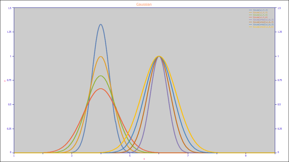
The Gaussian or normal peak with a0 as the peak amplitude is defined as follows:
a0 = Amplitude
a1 = Center (mean,mode,median)
a2 = Width (SD)
Built in model: Gauss[amp]
User-defined peaks and view functions: Gauss[amp](x,a0,a1,a2)
Lorentzian (Area)
The Lorentzian peak with a0 as the peak area is defined as follows:
a0 = Area
a1 = Center (mode)
a2 = Width
Built in model: Lorentz
User-defined peaks and view functions: Lorentz(x,a0,a1,a2)
Lorentzian (Amplitude)
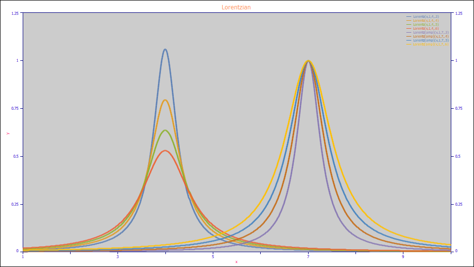
The Lorentzian peak with a0 as the peak amplitude is defined as follows:
a0 = Amplitude
a1 = Center (mode)
a2 = Width
Built in model: Lorentz[amp]
User-defined peaks and view functions: Lorentz[amp](x,a0,a1,a2)
Voigt (Area, Traditional Form)
The traditional Voigt peak with a0 as the peak area is defined as follows:
a0 = Area
a1 = Center (mode)
a2 = proportional to Gaussian Width
a3 = proportional to Lorentzian/Gaussian Width ratio
Built in model: Voigt
User-defined peaks and view functions: Voigt(x,a0,a1,a2,a3)
Voigt (Amplitude, Traditional)
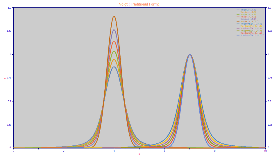
The traditional Voigt peak with a0 as the peak amplitude is defined as follows:
a0 = Amplitude
a1 = Center (mode)
a2 = proportional to Gaussian Width
a3 = proportional to Lorentzian/Gaussian Width ratio
Built in model: Voigt[amp]
User-defined peaks and view functions: Voigt[amp](x,a0,a1,a2,a3)
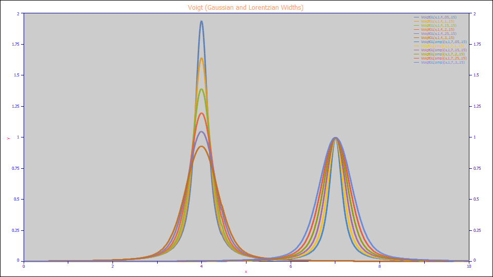
Voigt (Area, Gaussian and Lorentzian Widths)
The Voigt peak fitting the two widths directly with a0 as the peak area is defined as follows:
a0 = Area
a1 = Center (mode)
a2 = Gaussian Width (SD)
a3 = Lorentzian Width
Built in model: VoigtGL
User-defined peaks and view functions: VoigtGL(x,a0,a1,a2,a3)
Voigt (Amplitude, Gaussian and Lorentzian Widths)
The Voigt peak fitting the two widths directly with a0 as the peak amplitude is defined as follows:
a0 = Amplitude
a1 = Center (mode)
a2 = Gaussian Width (SD)
a3 = Lorentzian Width
Built in model: VoigtGL[amp]
User-defined peaks and view functions: VoigtGL[amp](x,a0,a1,a2,a3)
Generalized Voigt - Gaussian � Student's t (Area)
This is a Generalized Voigt which can be used to check the validity of the Voigt model assumption.
a0 = Area
a1 = Center
a2 = Gaussian Width
a3 = Lorentzian Width
a4 = Student's t nu (1=Lorentzian, Infinite=Gaussian)
Built in model: Gauss<S>
User-defined peaks and view functions: Gauss[S]i[amp](x,a0,a1,a2,a3) (Warning: computed as integral, very slow!)
![v5_Spectroscopy_Gauss[S]i.png](v5_Spectroscopy_Gauss[S]i.png)
Generalized Voigt - Lorentzian � Student's t (Area)
This is a Generalized Voigt which can be used to check the validity of the Voigt model assumption.
a0 = Area
a1 = Center
a2 = Lorentzian Width
a3 = Gaussian Width
a4 = Student's t nu (1=Lorentzian, Infinite=Gaussian)
Built in model:Lorentz<S>
User-defined peaks and view functions: Lorentz[S]i(x,a0,a1,a2,a3) (Warning: computed as integral, very slow!)
![v5_Spectroscopy_Lorentz[S]i.png](v5_Spectroscopy_Lorentz[S]i.png)
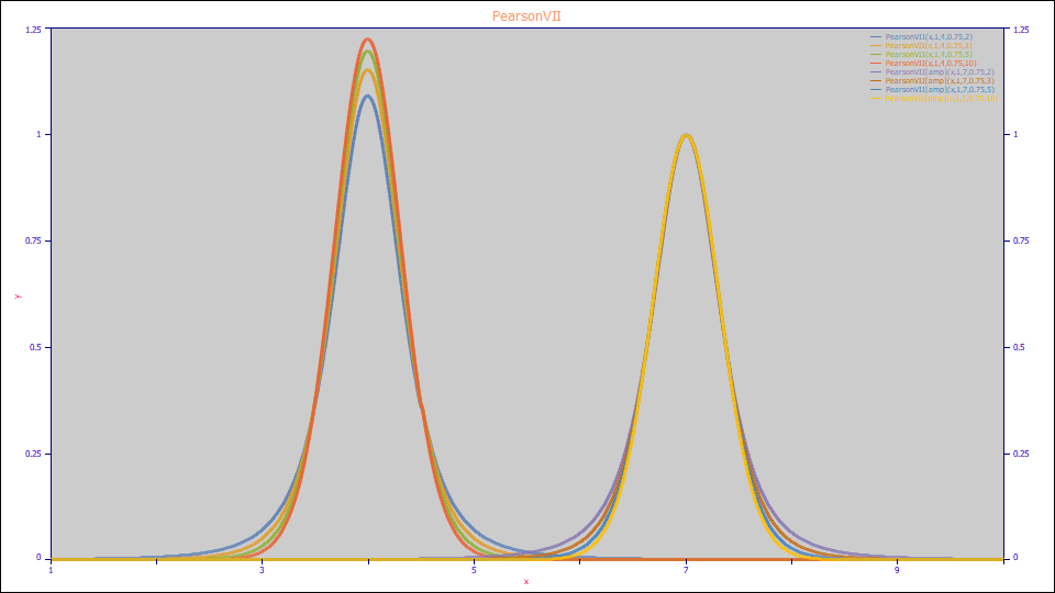
Pearson VII (Area)
The Pearson VII symmetric model with a0 as the peak area is defined as follows:
a0 = Area
a1 = Center (mode)
a2 = FWHM
a3 = Shape (1=Lorentzian, infinity=Gaussian)
Built in model: PearsonVII
User-defined peaks and view functions: PearsonVII(x,a0,a1,a2,a3)
Pearson VII (Amplitude)
The Pearson VII symmetric model with a0 as the peak amplitude is defined as follows:
a0 = Amplitude
a1 = Center (mode)
a2 = FWHM
a3 = Shape (1=Lorentzian, infinity=Gaussian)
Built in model:PearsonVII[amp]
User-defined peaks and view functions: PearsonVII[amp](x,a0,a1,a2,a3)
Sum Gaussian and Lorentzian (Area)
a0 = Area
a1 = Center (mode)
a2 = Width (FWHM)
a3 = Fraction Gaussian (0<a3<1)
Built in model: GLSum
User-defined peaks and view functions: GLSum(x,a0,a1,a2,a3)
Sum Gaussian and Lorentzian (Amplitude)
a0 = Amplitude
a1 = Center (mode)
a2 = Width (FWHM)
a3 = Fraction Gaussian (0<a3<1)
Built in model: GLSum[amp]
User-defined peaks and view functions: GLSum[amp](x,a0,a1,a2,a3)
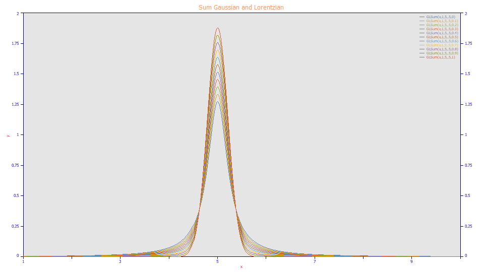
An approximation for the Voigt, this model simply sums equal FWHM Lorentzians and Gaussians. The parameter a directly computes the full-width at half-maximum (FWHM). The parameter a3 varies from 0 to 1, with 0 being a pure Lorentzian and 1 being a pure Gaussian.
Gaussian and Lorentzian "Cross Product" (Area)
a0 = Area
a1 = Center (mode)
a2 = Width
a3 = Fraction Gaussian (0<a3<1)
Built in model: GLProd
User-defined peaks and view functions: GLProd(x,a0,a1,a2,a3)
Gaussian and Lorentzian "Cross Product" (Amplitude)
a0 = Amplitude
a1 = Center (mode)
a2 = Width
a3 = Fraction Gaussian (0<a3<1)
Built in model: GLProd[amp]
User-defined peaks and view functions: GLProd[amp](x,a0,a1,a2,a3)
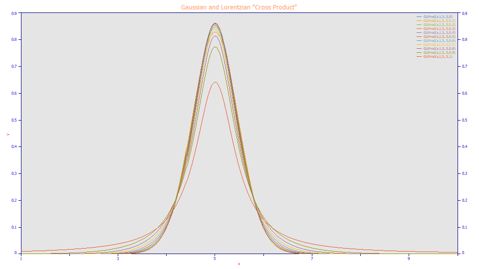
Another Voigt approximation, this model has been used for fitting XPS spectra. It combines the Gaussian and Lorentzian in a multiplicative format. As with the Gaussian-Lorentzian sum function, the a3 parameter varies from 0 to 1. Here though, the pure Lorentzian occurs with a3=1 and the pure Gaussian with an a3 =0. Another difference is that the degree of Lorentzian character is not a linear function of a3.
Constrained Gaussian (Area)
The Constrained Gaussian with a0 as the peak area is defined as follows:
a0 = Area
a1 = Center (mode)
a2 = width 1 (frequency invariant)
a3 = width 2 (frequency dependent)
Built in model: GaussCnstr
User-defined peaks and view functions: GaussCnstr(x,a0,a1,a2,a3)
Constrained Gaussian (Amplitude)
The Constrained Gaussian with a0 as the peak amplitude is defined as follows:
a0 = Amplitude
a1 = Center (mode)
a2 = width 1 (frequency invariant)
a3 = width 2 (frequency dependent)
Built in model:GaussCnstr[amp]
User-defined peaks and view functions: GaussCnstr[amp](x,a0,a1,a2,a3)
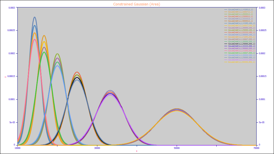
This model has no validity for fitting a single peak. The concept of this model is to fit many peaks with only two widths. The a2 width represents a constant line spread function, the width of each peak due to effects which have no frequency or energy dependence. The a3 term simply creates a scaled width which is linearly proportional to energy. It is not a width per se, but is used to produce a unique frequency-dependent width component for each peak. When fitting constrained Gaussians, a single a2 and a3 is always fit. Widths and shapes cannot be varied.
Gamma Ray Peak (Gaussian + Compton Edge)
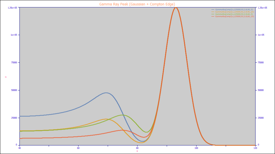
The Gamma Ray model combines an amplitude Gaussian with a Gaussian-smeared Compton edge function.
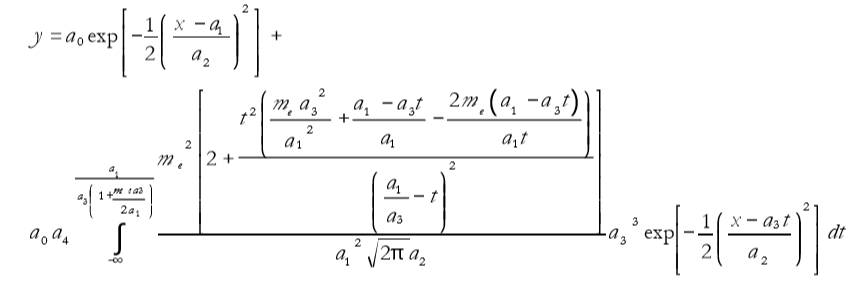
a0 = Amplitude (photopeak)
a1 = Center (energy photopeak and edge)
a2 = width (photopeak and edge smearing)
a3 = calibration (MeV/channels)
a4 = edge magnitude (as fraction of a0)
me = mass electron (.511004116)
Built in model:GammaRay
User-defined peaks and view functions: GammaRay(x,a0,a1,a2,a3,a4)
Compton Edge
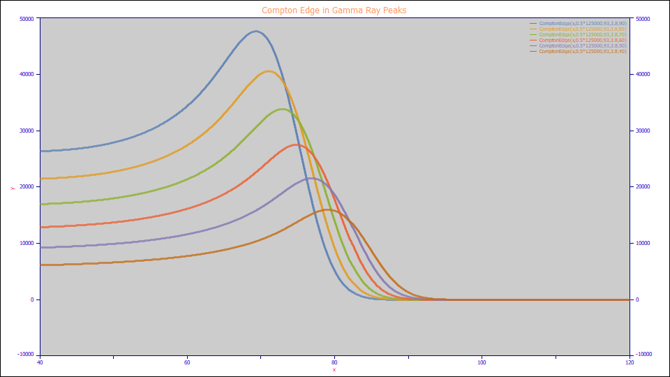
The Compton Edge model is defined as follows:

a0 = Amplitude edge magnitude
a1 = Center (energy edge)
a2 = width (edge smearing)
a3 = calibration (MeV/channels)
me = mass electron (.511004116)
Built in model:ComptonEdge
User-defined peaks and view functions: ComptonEdge(x,a0,a1,a2,a3)
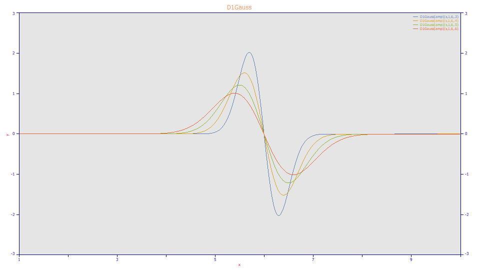
Gaussian First Derivative
a0 = Area
a1 = Center (mean,mode,median)
a2 = Width (SD)
Built in model: D1Gauss[amp]
User-defined peaks and view functions: D1Gauss[amp](x,a0,a1,a2)
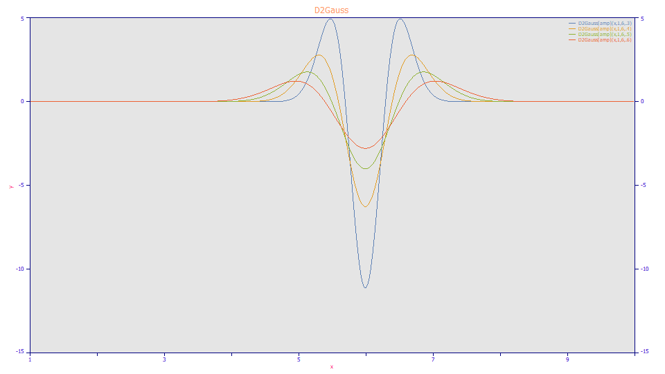
Gaussian Second Derivative
a0 = Area
a1 = Center (mean,mode,median)
a2 = Width (SD)
Built in model: D2Gauss[amp]
User-defined peaks and view functions: D2Gauss[amp](x,a0,a1,a2)
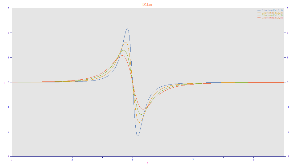
Lorentzian First Derivative
a0 = Area
a1 = Center (mode)
a2 = Width
Built in model: D1Lor[amp]
User-defined peaks and view functions: D1Lor[amp](x,a0,a1,a2)
Lorentzian Second Derivative
a0 = Area
a1 = Center (mode)
a2 = Width
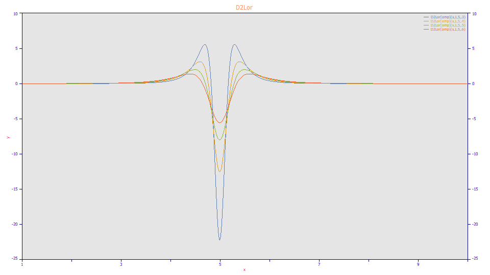
Built in model: D2Lor[amp]
User-defined peaks and view functions: D2Lor[amp](x,a0,a1,a2)
