PeakLab v1 Documentation Contents AIST Software Home AIST Software Support
White Paper: Part I - Generalized Chromatographic Models
Part I - Generalized Chromatographic Models
In this first white paper, we describe our discovery of an equivalence in chromatographic peak shapes relative to the concentration dependency in the HVL ((Haarhoff-Van der Linde) and Wade-Thomas NLC theoretical models. These are the two models we have found to be the far and away the most successful in modeling the nonlinear shapes that occur with chromatographic peaks. We then use this equivalence to develop generalized models which are capable of fitting the higher moments in chromatographic peaks, allowing high accuracy fits of LC, GC, HPLC and ultraHPLC (with and without gradients), and preparative or high overload,peaks. In this initial white paper, we cover the generalization of the models that describe the actual chromatographic separations as such applies to analytical peaks where only a third moment generalization is required.
In part II, we will address accounting the additional nonidealities in the chromatographic flow and detection systems. By adding an instrument response function in fitting a convolution model to chromatographic data, we will demonstrate analytic fits with less than 10 ppm least-squares error, and in certain instances, fit errors as low as 1 ppm. By using Fourier methods in the fitting, we will illustrate the performance to be suitable for routine analysis of chromatographic peaks.
In part III, we will specifically address gradient HPLC separations and the additional steps that must be taken to successfully estimate the gradient strength in the chromatographic modeling, this on a peak-by-peak basis. In covering gradient GHPLC fits, we will address twice-generalized chromatographic models which also address fourth moment adjustments.
In part IV, we will address the additional challenges of modeling overload shapes arising from preparative chromatography, estimating the peak shapes that would have been generated had the column had infinite capacity and no overload had taken place.
Peak Shapes in Chromatography
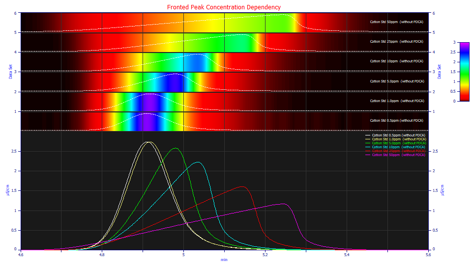
If a chromatographic peak is 'fronted', there is a progression in the strength of this fronting as concentration increases:

This plot of real-world data covers two orders of magnitude of concentration. The peaks are normalized to unit area. Note that the peaks at very low concentration show little apparent fronting, and even an unusual and appreciable tailing. The peaks show an increasingly right triangular fronted shape as concentration increases.
Similarly, if a chromatographic peak is 'tailed', there is a progression in the strength of this tailing as concentration increases:
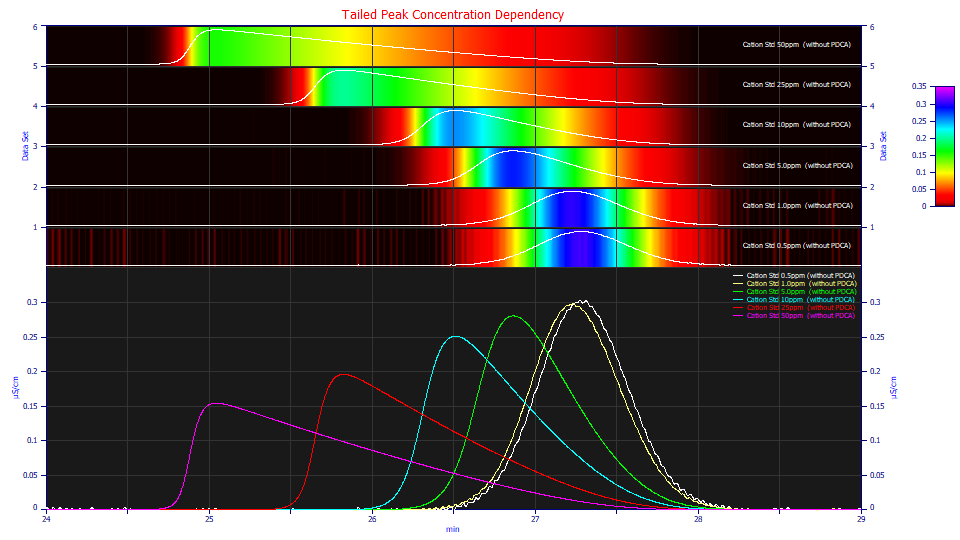
In the case of fronting, the higher concentration produces a later peak apex. In a tailed peak, the higher concentration produces an earlier apex.
It is this shape dependency with concentration that sets true chromatographic models apart from other density models. You can double the concetration, as in the progression from the green to blue peaks, and see appreciably different shapes.
The HVL Chromatographic Model
The Haarhoff-Van der Linde (ōHVLö) gas chromatography model is defined as follows:
(1)
If we look at the HVL as a statistical model absent its theoretical derivations, and in a form where the area is an adjustable parameter, we have a four parameter function. In this form, a0 is the peak area, a1 is the center or location value, a2 is the peak width or scale parameter, and a3 is the shape parameter, positive for a right-skewed asymmetry, negative for left-skewed. We have labeled the variables in the HVL model so that adjustable parameters a0-a3 correspond to moments 0-3.
The HVL produces a theoretical diffusion width, originally seen as applicable to GC, and was derived using adsorption isotherm arguments.
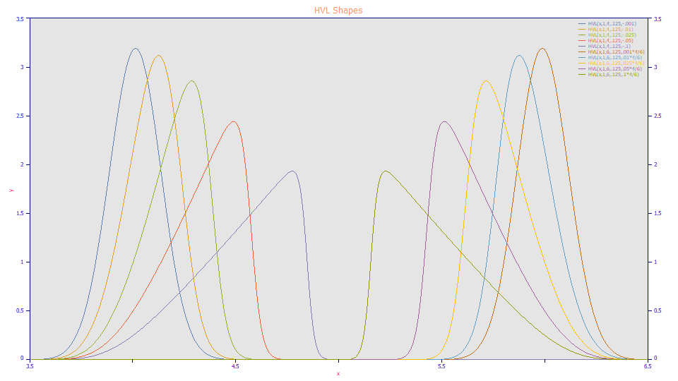
When the a3 distortion parameter is negative, the peaks are fronted; when positive, the peaks are tailed. In the HVL model, the a3 distortion is additionally scaled by a1/a2. The a3 values were adjusted for the a1 locations in the plot above to produce a mirroring, identical measures of fronting and tailing at the two different locations.
Note also the obvious issue with using an apex value for location when concentrations of a given solute can significantly vary. In this plot, the five fronted shapes would all fit to a 4.0 location and all five tailed shapes would fit to a 6.0 location. The same kind of issue applies to using a FWHM as a surrogate for the peak's second moment. In this case, all ten of the peaks in the plot will fit to a single .125 width, the SD of the underlying Gaussian when no distortion is present, the width at the limit of infinite dilution.
The NLC Chromatographic Model
The Wade-Thomas non-linear liquid chromatography model (ōNLCö) is defined as follows:
(2)
Where TFn is a modified Bessel function integral:
(3)
When the area is an adjustable parameter, the NLC is also a four parameter function. As with the HVL, a0 is the peak area and a1 is the center or location value, and a3 is the distortion parameter, positive for the right-skewed asymmetry of a tailed peak and negative for the left-skewed asymmetry of a fronted peak. This NLC parameterization uses a time constant instead of a rate constant for the a2 kinetic parameter given in the original publication of the Wade-Thomas NLC model. As such, the NLC a2 is similar to the HVL a2, a scale parameter that increases with the peak width.
The NLC produces a kinetic time constant, derived for LC when slow kinetics of adsorption and desorption are present, or where mass-transfer can be modeled by first order kinetics.
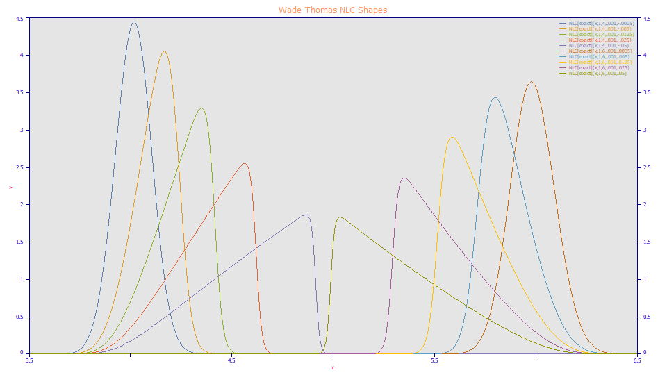
As with the HVL, when the NLC's a3 distortion parameter is negative, the peaks are fronted, and when positive, the peaks are tailed. In the NLC model, there is no additional scaling of the a3 distortion. The non-mirror shapes with identical magnitude a3 values are from the asymmetry in the underlying Giddings kinetic model which the NLC generates at the infinite dilution (zero concentration) limit.
Here as well using the apex and FWHM values is fraught with error with respect to concentration independent estimates of the location and broadening, or the first and second moments. All ten of these NLC shapes fit to the same a2 time constant. The five fronted NLC shapes fit to a 4.0 a1 center value and the five tailed shapes each fit to a 6.0 a1 value. These are the mean of the underlying (zero distortion) Giddings density.
Note also that the 0.001 first order time constant value used in these plots represents exceptionally fast kinetics, and yet the shapes track the real-world data in the initial concentration plots.
The Generalized HVL Template
The HVL reduces to a Gaussian at infinite dilution. We will first generalize the HVL model, using the Gaussian or normal probability density function (PDF):
(4)
We also use the Gaussian or normal cumulative distribution function (CDF):
(5)
We also take note of the complement of the CDF, the reverse cumulative of the normal density, even though it is not used in the HVL:
(6)
We can now rewrite the HVL as a generalized template that accepts any zero-distortion density:
(7)
To regenerate the HVL, Density is replaced with (4), the normal PDF, and Cumulative with (5), the normal CDF. Note that any replacement is always done with a matched PDF-CDF (Density-Cumulative) pair.
The Generalized NLC Template
To create a generalized NLC model template, we use the Giddings density:
(8)
Here we take note of the Giddings cumulative, although it is not used in the NLC:
(9)
We also use the Giddings reverse cumulative:
(10)
The NLC generalized density template can then be expressed as follows:
(11)
Just as with the HVL template, we can create any number of NLC-based generalized models by inserting a matched density-cumulative pair other than the Giddings for the zero-distortion assumption.
To regenerate the NLC, Density is replaced with (8), the Giddings PDF, and RevCumulative with (10), the Giddings CDF complement.
The Common Chromatographic Distortion Model
Despite different derivations across decades which targeted different types of chromatography, the generalized templates of the two models produce identical shapes for a given density-cumulative pair.
One can substitute the Gaussian PDF and CDF complement in the NLC template and exactly generate a shape that is exactly fitted by the HVL model. Similarly the Giddings PDF and CDF can be inserted into the HVL template to produce a shape that is exactly fitted by the Wade-Thomas NLC model.
Note that the a1 associated with the first moment, and the a2 associated with the second moment, also appear in the templates, and while the a1 center values are comparable (both represent the mean of the underlying ZDD), the a2's consist of immensely different representations of the peak broadening, one a Gaussian diffusion width, the other a Giddings kinetic time constant associated with adsorption-desorption.
Apart from the distortion scaling in the HVL and the use of the CDF in the HVL and the CDF complement in the NLC, the only difference between the HVL and NLC models is their zero-distortion density assumption. The HVL assumes a diffusion-based Gaussian, the simplest possible probabilistic density assumption. The NLC assumes a first order Giddings density, the simplest kinetic density assumption possible.
If you have long used both the HVL and NLC models in fitting chromatographic peaks, you were probably struck by the similarities in the fits. Part of this can be attributed to the similarity between the Gaussian and Giddings zero-distortion densities:
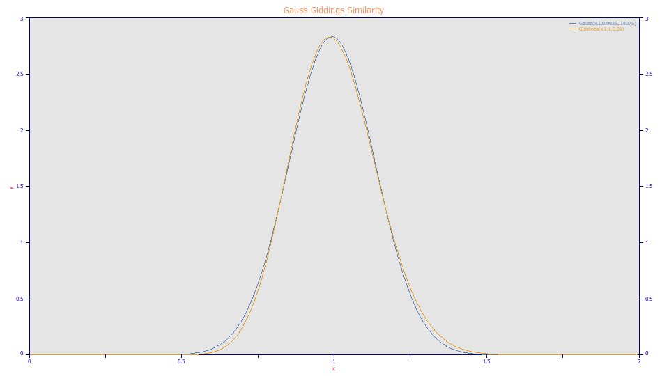
The Giddings density, the amber curve, is a slightly right-asymmetric peak as compared to the symmetric Gaussian, the blue curve. This symmetry explains why the HVL produces mirrored shapes about a1 with negative distortions, whereas the NLC produces different tailed and fronted shapes with the same magnitude of the a3 distortion parameter.
Extending the HVL and NLC Generalized Templates to Fit Higher Moments in Chromatographic Peaks
The major drawback of the basic HVL and NLC models is that the higher moments are fixed by the Gaussian and Giddings zero-distortion assumptions. Any non-ideality in the chromatographic separation, such as multiple-site adsorptions in the kinetic model, or asymmetry in the diffusion model are not accommodated.
The HVL and NLC generalized templates allow for any density-cumulative pair to be used. The zero distortion density (ZDD) need not have fixed higher moments as locked in by the Gaussian or Giddings assumptions. To create generalized HVL and NLC models, all that is needed is to assume the ZDD is neither Gaussian or Giddings but a more complex density that allows for the third moment, the skewness, to be broadly adjustable. This is what we refer to as a once-generalized model, the addition of third moment or skewness adjustments. Only if one is addressing gradient HPLC or overloaded preparative shapes, is a twice-generalized model, one which also allows for adjustments in the kurtosis (fourth moment, fatness of tails), needed.
By reducing the generalization problem to the zero concentration limiting density, there is an immense simplification, one readily addressed by the statistical sciences. In order to create a once-generalized HVL or NLC, we can use any one of a number of generalized Gaussians where third and/or fourth moments are adjustable. The generalization problem is thus rendered the straightforward one of finding a ZDD which would readily fit HVL and NLC shapes as two families of curves determined by two specific values of a third moment skewness parameter. Given the unlimited possibilities of skewness, such a generalization would also model every chromatographic shape where a skewness was introduced into the infinite dilution density.
A major benefit of a once-generalized closed-form model is an immense simplification of the NLC shape. If the generalization can accurately replicate the Giddings shape, the need for the modified Bessel approximation, and the far more computationally demanding modified Bessel function integral, both of which make the computation of the NLC so onerous, will cease to exist. The NLC shapes will simply be one of the infinite families of shapes the generalized models can produce, the HVL another.
Generalized Default ZDD (One Higher Moment)
We can adopt the widely used asymmetric generalized normal as the density in the templates. This density is not defined at all x, but it is computationally easy to compute:
a0 = Area
a1 = Center (as mean of asymmetric peak)
a2 = Width (SD of underlying Gaussian)
a3 = Asymmetry ( fronted -1 > a3 > 1 tailed)
GenHVL - Default Generalized Normal ZDD
If we substitute this statistical PDF and its CDF into the HVL template for tailed shapes, and this same PDF and its CDF complement into the NLC for fronted shapes, we can construct the Generalized HVL model for chromatography:
a0 = Area
a1 = Center (as mean of asymmetric peak)
a2 = Width (SD of underlying Gaussian ZDD)
a3 = HVL Chromatographic distortion ( -1 > a3 > 1 )
a4 = ZDD asymmetry ( -1 > a4 > 1 )
Note that the a4 value controlling the skew of the GenHVL peak appears as a3 in the ZDD nomenclature.
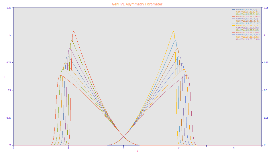
The once-generalized HVL model, and the once generalized NLC model produce identical shapes, and both reproduce the HVL to full precision and the NLC to 6-8 digits precision. The GenHVL model reports a diffusion width for a2 and a statistical asymmetry for the a4 parameter. The GenNLC differs only in parameterization, reporting a first order kinetic time constant for a2 and an asymmetry indexed to the Giddings/NLC for a4.
An Example of Fitting the GenHVL to Real-World Data
Even though we have a generalized model for the chromatographic separation which accounts a third moment skewness in the infinite dilution density, we have not as yet accounted the real-world non-idealities in a chromatographic system. We will cover this in the next paper in this series. For this illustration, we will jump ahead somewhat and remove the IRF (instrument response function) prior to fitting the GenHVL to a real-world set of IC data standards containing a mix of appreciably fronted and tailed peaks. We thus remove the instrument and system distortions prior to fitting with a Fourier deconvolution procedure that uses values estimated in an IRF determination which quantifies the non-idealities in the flow path and detection.
One of the largest tradeoffs in chromatographic modeling is in using a low enough concentration to see mostly Gaussian peaks and still having a high enough S/N to get effective fits on all components of interest. If one has a model which is capable of managing distorted shapes and reporting true theoretical location and broadening values, independent of concentration, then one can fit the more distorted shapes in a higher concentration sample and benefit from the improved S/N in the data.
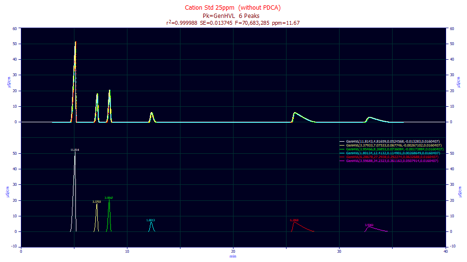
Despite the additional noise introduced by the Fourier deconvolution, this high S/N sample, with the higher concentration fronting and tailing, fit to just 11 ppm least squares error. The following analytical fits are for three different concentrations of the above standard.
"CationĀStdĀ5.0ppmĀĀ(withoutĀPDCA)"
FittedĀParameters
r2ĀCoefĀDetĀĀ DFĀAdjĀr2ĀĀĀĀ FitĀStdĀErrĀĀ F-valueĀĀĀĀĀĀ ppmĀuVar
0.99996468ĀĀĀ 0.99996464ĀĀĀ 0.00611751ĀĀĀ 23,348,983ĀĀĀ 35.3179206
ĀPeakĀĀ TypeĀĀĀĀ ĀĀĀĀĀĀa0ĀĀĀĀ ĀĀĀĀĀĀa1ĀĀĀĀ ĀĀĀĀĀĀa2ĀĀĀĀ ĀĀĀĀĀĀa3ĀĀĀĀ ĀĀĀĀĀĀa4ĀĀĀĀ
ĀĀĀĀ1ĀĀ GenHVLĀĀ 2.39409195ĀĀ 4.86629842ĀĀ 0.04836896ĀĀ -0.0028304ĀĀ 0.01010560ĀĀ
ĀĀĀĀ2ĀĀ GenHVLĀĀ 0.68483314ĀĀ 7.09399421ĀĀ 0.06635864ĀĀ -0.0005339ĀĀ 0.01010560ĀĀ
ĀĀĀĀ3ĀĀ GenHVLĀĀ 0.79975294ĀĀ 8.27604890ĀĀ 0.07330294ĀĀ -0.0003202ĀĀ 0.01010560ĀĀ
ĀĀĀĀ4ĀĀ GenHVLĀĀ 0.36554694ĀĀ 12.3963875ĀĀ 0.11414019ĀĀ 0.00043770ĀĀ 0.01010560ĀĀ
ĀĀĀĀ5ĀĀ GenHVLĀĀ 1.27705415ĀĀ 27.3145721ĀĀ 0.27360663ĀĀ 0.01257608ĀĀ 0.01010560ĀĀ
ĀĀĀĀ6ĀĀ GenHVLĀĀ 0.72539077ĀĀ 34.1882845ĀĀ 0.33736125ĀĀ 0.00969516ĀĀ 0.01010560ĀĀ
MeasuredĀValues
ĀPeakĀĀ TypeĀĀĀĀ ĀAmplitudeĀĀ ĀĀCenterĀĀĀĀ ĀĀĀFWHMĀĀĀĀĀ ĀĀAsym50ĀĀĀĀ ĀFWĀBaseĀĀĀĀ ĀĀAsym10ĀĀĀĀ
ĀĀĀĀ1ĀĀ GenHVLĀĀ 17.5378848ĀĀ 4.96975730ĀĀ 0.12879519ĀĀ 0.51112283ĀĀ 0.26013732ĀĀ 0.44708895ĀĀ
ĀĀĀĀ2ĀĀ GenHVLĀĀ 4.09186251ĀĀ 7.11573005ĀĀ 0.15730496ĀĀ 0.90616835ĀĀ 0.31466816ĀĀ 0.88988455ĀĀ
ĀĀĀĀ3ĀĀ GenHVLĀĀ 4.34018865ĀĀ 8.28935683ĀĀ 0.17315652ĀĀ 0.94978109ĀĀ 0.34642154ĀĀ 0.94378805ĀĀ
ĀĀĀĀ4ĀĀ GenHVLĀĀ 1.27903707ĀĀ 12.3757241ĀĀ 0.26840030ĀĀ 1.06764105ĀĀ 0.53777053ĀĀ 1.09299830ĀĀ
ĀĀĀĀ5ĀĀ GenHVLĀĀ 1.77534645ĀĀ 26.8452258ĀĀ 0.67323521ĀĀ 1.75253266ĀĀ 1.37786763ĀĀ 2.01359269ĀĀ
ĀĀĀĀ6ĀĀ GenHVLĀĀ 0.84270757ĀĀ 33.8047084ĀĀ 0.80653519ĀĀ 1.45452305ĀĀ 1.63450870ĀĀ 1.60664078ĀĀ
"CationĀStdĀ10ppmĀĀ(withoutĀPDCA)"
FittedĀParameters
r2ĀCoefĀDetĀĀ DFĀAdjĀr2ĀĀĀĀ FitĀStdĀErrĀĀ F-valueĀĀĀĀĀĀ ppmĀuVar
0.99998410ĀĀĀ 0.99998408ĀĀĀ 0.00756954ĀĀĀ 51,856,486ĀĀĀ 15.9026113
ĀPeakĀĀ TypeĀĀĀĀ ĀĀĀĀĀĀa0ĀĀĀĀ ĀĀĀĀĀĀa1ĀĀĀĀ ĀĀĀĀĀĀa2ĀĀĀĀ ĀĀĀĀĀĀa3ĀĀĀĀ ĀĀĀĀĀĀa4ĀĀĀĀ
ĀĀĀĀ1ĀĀ GenHVLĀĀ 4.76595940ĀĀ 4.84877877ĀĀ 0.04839938ĀĀ -0.0054830ĀĀ 0.01425771ĀĀ
ĀĀĀĀ2ĀĀ GenHVLĀĀ 1.36140311ĀĀ 7.08591237ĀĀ 0.06632691ĀĀ -0.0010553ĀĀ 0.01425771ĀĀ
ĀĀĀĀ3ĀĀ GenHVLĀĀ 1.59490007ĀĀ 8.26994645ĀĀ 0.07297309ĀĀ -0.0006439ĀĀ 0.01425771ĀĀ
ĀĀĀĀ4ĀĀ GenHVLĀĀ 0.72807999ĀĀ 12.3913245ĀĀ 0.11433678ĀĀ 0.00099639ĀĀ 0.01425771ĀĀ
ĀĀĀĀ5ĀĀ GenHVLĀĀ 2.53401578ĀĀ 27.3046832ĀĀ 0.27963325ĀĀ 0.02528927ĀĀ 0.01425771ĀĀ
ĀĀĀĀ6ĀĀ GenHVLĀĀ 1.45127017ĀĀ 34.1888513ĀĀ 0.34552620ĀĀ 0.01984923ĀĀ 0.01425771ĀĀ
MeasuredĀValues
ĀPeakĀĀ TypeĀĀĀĀ ĀAmplitudeĀĀ ĀĀCenterĀĀĀĀ ĀĀĀFWHMĀĀĀĀĀ ĀĀAsym50ĀĀĀĀ ĀFWĀBaseĀĀĀĀ ĀĀAsym10ĀĀĀĀ
ĀĀĀĀ1ĀĀ GenHVLĀĀ 29.5298652ĀĀ 5.02552694ĀĀ 0.15434218ĀĀ 0.33255295ĀĀ 0.30954552ĀĀ 0.28134430ĀĀ
ĀĀĀĀ2ĀĀ GenHVLĀĀ 8.02653978ĀĀ 7.12919908ĀĀ 0.15955211ĀĀ 0.81889325ĀĀ 0.31899002ĀĀ 0.78692972ĀĀ
ĀĀĀĀ3ĀĀ GenHVLĀĀ 8.63873996ĀĀ 8.29746430ĀĀ 0.17358139ĀĀ 0.89449898ĀĀ 0.34700759ĀĀ 0.87811423ĀĀ
ĀĀĀĀ4ĀĀ GenHVLĀĀ 2.54584420ĀĀ 12.3460701ĀĀ 0.26838043ĀĀ 1.14773956ĀĀ 0.53899929ĀĀ 1.20028957ĀĀ
ĀĀĀĀ5ĀĀ GenHVLĀĀ 3.17348807ĀĀ 26.4873173ĀĀ 0.74615841ĀĀ 2.57612679ĀĀ 1.56417775ĀĀ 3.16318080ĀĀ
ĀĀĀĀ6ĀĀ GenHVLĀĀ 1.57429789ĀĀ 33.4774236ĀĀ 0.86111357ĀĀ 1.96515093ĀĀ 1.77985289ĀĀ 2.31704802ĀĀ
"CationĀStdĀ25ppmĀĀ(withoutĀPDCA)"
FittedĀParameters
r2ĀCoefĀDetĀĀ DFĀAdjĀr2ĀĀĀĀ FitĀStdĀErrĀĀ F-valueĀĀĀĀĀĀ ppmĀuVar
0.99998833ĀĀĀ 0.99998832ĀĀĀ 0.01374504ĀĀĀ 70,683,285ĀĀĀ 11.6669314
ĀPeakĀĀ TypeĀĀĀĀ ĀĀĀĀĀĀa0ĀĀĀĀ ĀĀĀĀĀĀa1ĀĀĀĀ ĀĀĀĀĀĀa2ĀĀĀĀ ĀĀĀĀĀĀa3ĀĀĀĀ ĀĀĀĀĀĀa4ĀĀĀĀ
ĀĀĀĀ1ĀĀ GenHVLĀĀ 11.8142696ĀĀ 4.81659065ĀĀ 0.05245682ĀĀ -0.0132830ĀĀ 0.01604070ĀĀ
ĀĀĀĀ2ĀĀ GenHVLĀĀ 3.37933473ĀĀ 7.07533282ĀĀ 0.06774599ĀĀ -0.0026710ĀĀ 0.01604070ĀĀ
ĀĀĀĀ3ĀĀ GenHVLĀĀ 3.95466006ĀĀ 8.26853142ĀĀ 0.07360840ĀĀ -0.0017388ĀĀ 0.01604070ĀĀ
ĀĀĀĀ4ĀĀ GenHVLĀĀ 1.80133596ĀĀ 12.4132466ĀĀ 0.11490052ĀĀ 0.00268649ĀĀ 0.01604070ĀĀ
ĀĀĀĀ5ĀĀ GenHVLĀĀ 6.28678029ĀĀ 27.2937733ĀĀ 0.29227426ĀĀ 0.06326881ĀĀ 0.01604070ĀĀ
ĀĀĀĀ6ĀĀ GenHVLĀĀ 3.59687759ĀĀ 34.2322923ĀĀ 0.36116313ĀĀ 0.05079139ĀĀ 0.01604070ĀĀ
MeasuredĀValues
ĀPeakĀĀ TypeĀĀĀĀ ĀAmplitudeĀĀ ĀĀCenterĀĀĀĀ ĀĀĀFWHMĀĀĀĀĀ ĀĀAsym50ĀĀĀĀ ĀFWĀBaseĀĀĀĀ ĀĀAsym10ĀĀĀĀ
ĀĀĀĀ1ĀĀ GenHVLĀĀ 51.3969315ĀĀ 5.13548306ĀĀ 0.22524705ĀĀ 0.18947414ĀĀ 0.43971849ĀĀ 0.15866465ĀĀ
ĀĀĀĀ2ĀĀ GenHVLĀĀ 18.3887055ĀĀ 7.18040938ĀĀ 0.17331581ĀĀ 0.61719324ĀĀ 0.34737404ĀĀ 0.55997115ĀĀ
ĀĀĀĀ3ĀĀ GenHVLĀĀ 20.5719358ĀĀ 8.34339547ĀĀ 0.18101521ĀĀ 0.73016511ĀĀ 0.36202471ĀĀ 0.68469431ĀĀ
ĀĀĀĀ4ĀĀ GenHVLĀĀ 6.21391502ĀĀ 12.2981959ĀĀ 0.27141977ĀĀ 1.39865836ĀĀ 0.55027979ĀĀ 1.53839159ĀĀ
ĀĀĀĀ5ĀĀ GenHVLĀĀ 6.17339933ĀĀ 25.7952864ĀĀ 0.95570974ĀĀ 4.78387753ĀĀ 2.05567140ĀĀ 6.26432429ĀĀ
ĀĀĀĀ6ĀĀ GenHVLĀĀ 3.20405947ĀĀ 32.8180426ĀĀ 1.05023079ĀĀ 3.46401927ĀĀ 2.23464512ĀĀ 4.40839341ĀĀ
Additive-free cation standards were processed at 5, 10, and 25 ppm concentration. The analysis consists of strongly baseline-resolved peaks with highly fronted and tailed peaks at the higher concentrations. Here we answer why one would want to engage the extra effort to mathematically model chromatographic peaks. Let us assume it might be perfectly expected that a solute of interest would vary by a factor of five in its presence in a sample. If you look at the apex values for the first peak, you see that its values change from 4.970 to 5.125 with concentration. The last peak in the standard changes from 33.805 to 32.818. With respect to FWHM values the first peak varies from .129 to .225 and the last peak varies from .806 to 1.05 with the increasing concentration.
If we look at the a1 fitted values, the center of the infinite dilution Gaussian, we see close to concentration independence. The first peak varies from 4.866 to 4.816, and the last from 34.188 to 34.232, across the 5x increase in concentration. If we look at the a2 fitted values, the standard deviation of this infinite dilution Gaussian, the first peak varies from .0484 to .0524, and the last from .337 to .361. The coefficient of variation for the a1 fitted values averages .15%. For the a2 widths, it is 2.26%. By contrast, the CV for the center or apex values varies 1.06% and the FWHM values vary 11.8%.
Fitting baseline resolved peaks does more than just remove concentration effects from location and broadening estimates. The a3 parameter estimates the measure of fronting or tailing, and a3/a0 will actually offer a concentration independent estimate of the fronted or tailed distortion in any given peak. The higher moment a4 parameter, the skewness in the infinite dilution generalized Gaussian, increases with concentration in this example, something that would perhaps be expected if this parameter were estimating the measure of additional site adsorptions or collision effects and those were nonlinear with concentration. The various parametric estimates tell you much more about each peak, and further, when fits are this accurate, these five fitted parameters can completely reconstruct each peak, as shown in the lower portion of the fitted plot.
White Paper: Part II - Instrument Response Convolution Models
In this white paper, we looked only at the enhancements necessary to fully model the actual chromatographic separation, and only for analytic peaks where one higher third moment adjustment suffices to capture virtually all of the variance in the fitting. We have described a generalized HVL which is capable of fitting all HVL and NLC shapes as well as those of any other third moment asymmetry in the infinite dilution ZDD.
Fitting the third moment skewness in the infinite dilution ZDD is important, but for most chromatographic fitting, this removal of instrumental effects will typically be of greater significance in producing near zero-error fits. In the data above, we removed the instrumental/system distortions prior to fitting and realized fits with 35, 16, and 12 ppm error using this once-generalized HVL model. If the IRF is not pre-subtracted, and a pure HVL is fit to this same data, this forced Gaussian ZDD assumption and no modeling of the IRF results in much higher 2587, 2751, and 2414 ppm errors. To effectively fit chromatographic peaks, this higher moment generalization and an accounting of the instrumental distortions are both necessary.
In part II, we will describe the fitting of the real-world non-idealities in chromatographic data using convolution models.