PeakLab v1 Documentation Contents AIST Software Home AIST Software Support
White Paper: Part IV - Fitting Preparative (Overload) Peaks
Part IV - Preparative (Overload) Peaks
In Part I of this series we described a generalization of the HVL and NLC models which accommodated higher moment differences in the zero distortion (infinite dilution) density underlying the peak shapes in chromatographic separations. In Part II, we added the complexity of fitting the mathematical convolution of this 'true' peak model and an IRF, or instrument response function, in the fitting of analytical isocratic peaks. In Part III, we addressed the further complication in the shape of chromatographic peaks when the strength of the mobile phase is changing in gradient HPLC separations. In Part IV, we will now address the sharply different chromatographic shapes which occur when the concentrations are high and major column overload is present.
The Challenge of Fitting Overload Shapes
Of all the types of chromatographic peak shapes, preparative or overload profiles have proven to be the most challenging to fit to the near zero error we see in the other types of chromatography. In an overload peak, the eluted shapes arise from the column and/or the detector function being saturated. In effect, the expected peaks are nowhere seen because of a breakdown in either the separation in the column, the signal response in the detector, or both. The high amount of eluting solute is processed very differently in this condition of saturation.
We have discovered overload models that are true theoretical chromatographic convolution models which address this saturation or breakdown and can reconstruct the peaks that would have been seen if the column and detector could fully manage infinite concentrations, as if having infinite capacity and response.
In fact, the same third and fourth moment twice-generalized models used in directly fitting the gradient shapes, as was done in Part III of this white paper series, are effective in fitting preparative shapes. There is one important difference. With HPLC gradient peaks, we treat the gradient as a compression in the fourth moment of the ZDD, or zero-distortion density. For overload shapes, it is the opposite, a dilation of the tails in the ZDD. Instead of fitting a higher power of fourth moment-related decay that represents a compression, we fit a lower power of fourth moment-related decay that represents a dilation of the tails. This dilation in the ZDD's tails manages this overload state and produces the overload shapes seen in preparative chromatography.
Just as with fitting constant mobile phase analytic peaks, IRF tailing must be addressed by fitting an IRF-bearing model, a convolution integral. Although we can modify the ZDD zero distortion density with this power of decay dilation to produce the overall core shape of the overload envelope, we cannot manage the high measure of instrumental/system distortion without fitting an <irf> convolution integral. With preparative shapes, a convolution integral is non-optional.
We also know that multiple non-idealities in fluid flow, mass transfer, and detection enter into the IRF components. We know that even the two component <ge>, <e2>, and <pe> IRFs we routinely use for analytic peaks represent simplifications that will not fully capture the error arising from all of these different distortions or non-idealities. If the tailing arising from the IRF in preparative shapes is much increased by this overload state, we would expect any error in fitting the IRF portion of the peak's tailing to likewise be amplified.
Overload Shapes
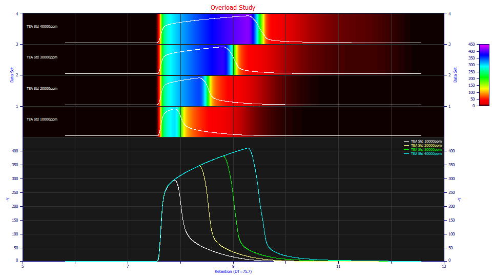
The following data consist of four TEA (triethanolamine) overload peaks with concentrations varying between 1 and 4 % (10000, 20000, 30000, and 40000 ppm in the titles). The dead time transform and baseline correction have already been applied.

Both the contour and non-normalized data plots clearly confirm the overload state. The additional concentration goes into the overload envelope. Note the differences in the strong tailing. If you were to place a tangent line on the decay of each of the envelopes, you see the tailing beginning at about 140, 110, 95, and 70 Y signal values across the four samples. If we treat this tailing as an IRF, the exposed portion of the IRF is greatest on the lowest concentration sample, and smallest on the highest concentration sample. If you look at the area-normalized contours, the tailing appears more drawn out for the higher concentration samples. The tailing is important because fitting the IRF is essential in accurately modeling overload peaks.
The GenHVL[Yp] Overload Model
The twice generalized Gen2HVL (fitting both third moment and fourth moment effects), covered in Part III of this white paper series, effectively manages these overload shapes. The Gen2HVL model's ZDD (zero distortion density) defines the a1 location parameter as the mean of the generalized error ZDD. The [Y] ZDD retains the a1 as the mean of the underlying Gaussian and we have chosen to use this form of the [Y] ZDD for the overload models:
a0 = Area
a1 = Center
a2 = Width
a3= Error model power (.25 > a3 > 4 , Laplace=1, Gaussian=2)
a4 = Asymmetry ( fronted -1 > a4 > 1 tailed)
When the power of decay (the fourth moment a3 term above) in the [Y] generalized error class of ZDD drops from 2.0 toward 1.0, this dilation produces a progression similar to those in the sequence above. In fact, by the time an 'envelope' has fully formed, this fourth moment decay parameter fits to very close to 1.0, a ZDD which decays as a double-sided exponential or Laplace density.
By inserting this [Y] Generalized Error Model ZDD for the PDF, CDF, and CDFc in the GenHVL template, we produce the GenHVL[Y] model. The GenHVL[Yp] (the appended 'p' for 'preparative') is identical to the GenHVL[Y] but offers a different starting estimate algorithm which assumes a high overload shape. In order to ensure the convergence of the non-linear fitting to an optimal solution, the starting estimates must be specific for this condition of overload. The GenHVL[Yp] model is as follows:
a0 = Area
a1 = Center (as mean of underlying normal ZDD)
a2 = Width (SD of underlying normal ZDD)
a3 = HVL Chromatographic distortion ( -1 > a3 > 1 )
a4 = Power n in exp(-zn) decay ( .25 > a4 > 4 ) adjusts kurtosis (fourth moment)
a5 = ZDD asymmetry ( -1 > a5 > 1 ), adjusts skew (third moment)
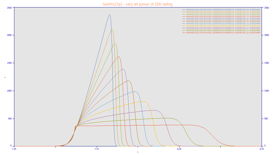
When the a4 power of tail decay in the ZDD of the GenHVL[Yp] model is 2.0, the generalized HVL peak is generated (the blue peak which has a traditional chromatographic peak shape). As the a4 power decreases to the 1.0 of double-sided exponential or Laplace type of decay, the shape markedly changes as an overload envelope forms. Strongly overload preparatory shapes will have an a4 value very close to 1.0.
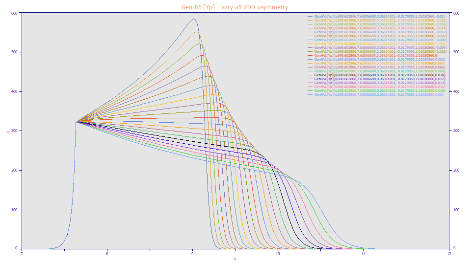
The a5 ZDD asymmetry primarily impacts the slope of the envelope when a high overload shape (a4 approaching 1.0) is present. The most negative a5 value in the plot above produces the sharpest upward slope for the envelope. The most positive of the a5 values produces the sharpest downward slope in the envelope.
It is important to note that all of this overload model is a theoretical generalized chromatographic model which uses the common chromatographic distortion mathematics, just as was true of the models used in all of the other types of chromatographic peaks. In fact, with the proper starting estimates, this [Y] generalized error twice-generalized class of ZDD, can successfully fit virtually any chromatographic shape: analytic GC and LC peaks, gradient HPLC peaks, and overload preparative peaks. This two-higher moment class of chromatographic model could easily be deemed a universal model were it not for the fact the analytic peaks generally require only a third moment adjustment.
The GenHVL[Yp2] Overload Model
If one assumes there are two distinct behaviors in the formation of an overload shape, one prior to the apex of the underlying zero distortion density, and one after, and one is constructing a model that will be used near to this a5=1.0 high overload envelope where there already exists a sharp reversal in slope at the apex, it is a straightforward matter to create a two-width ZDD, one width used only for the rise or left side of the ZDD, the other only for the decay or right side of the ZDD. This offers a much greater control of the initial rise of the overload shape.
The GenHVL[Yp2] model is this modification of the GenHVL[Yp] where there are two widths fitted, a width for the ZDD peak consisting of the rise to the apex, and a separate width for the ZDD peak which decays from the apex. Although an additional parameter is required, this model can often be fitted successfully, and often with much better goodness of fits. With two components, one pre-apex, one post-apex, the ZDD is going to necessarily be more complicated. The [Yp2] ZDD is defined as follows:
a0 = Area
a1 = Center
a2 = Width
a3 = Width Asymmetry (right side width)/(left side width)
a4 = Error model power (.25 > a4
> 4 , Laplace=1, Gaussian=2)
a5 =
Statistical Asymmetry ( fronted -1 > a5
> 1 tailed)
By inserting this [Yp2] Generalized Error 2-width Model ZDD for the PDF, CDF, and CDFc in the GenHVL template, we produce the GenHVL[Yp2] model:
a0 = Area
a1 = Center (as mean of underlying normal ZDD)
a2 = Width (SD of underlying normal ZDD)
a3 = HVL Chromatographic distortion ( -1 > a3
> 1 )
a4 = Width Asymmetry
(right side width)/(left side width)
a5 = Power
n in exp(-zn) decay ( .25 > a5
> 4 ) adjusts kurtosis (fourth moment)
a6 = ZDD asymmetry ( -1 > a6 > 1 ), adjusts skew (third moment)
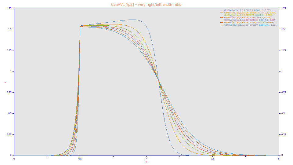
In this model, a4 is now the ZDD width ratio (right/Left), a5 is the ZDD power of decay, and a6 is the ZDD asymmetry. The plot above illustrates the impact of separate rise and decay widths. The overall a2 width was adjusted across the shapes to produce approximately the same envelope width and inflection point. Here the right/left width ratio is varied from 1.0, the curve with the softest rise and the most positive slope in the envelope, to 10.0, the curve with the sharpest rise and the most negative slope in the envelope. The two-width model primarily adds the ability to adjust the sharpness of the rise in the overload shape.
Fitting the Single-Width GenHVL[Yp]<e2> Model
If the four TEA data sets are fitted to the single width twice-generalized HVL with the two-component exponential IRF, the fits hare as follows:
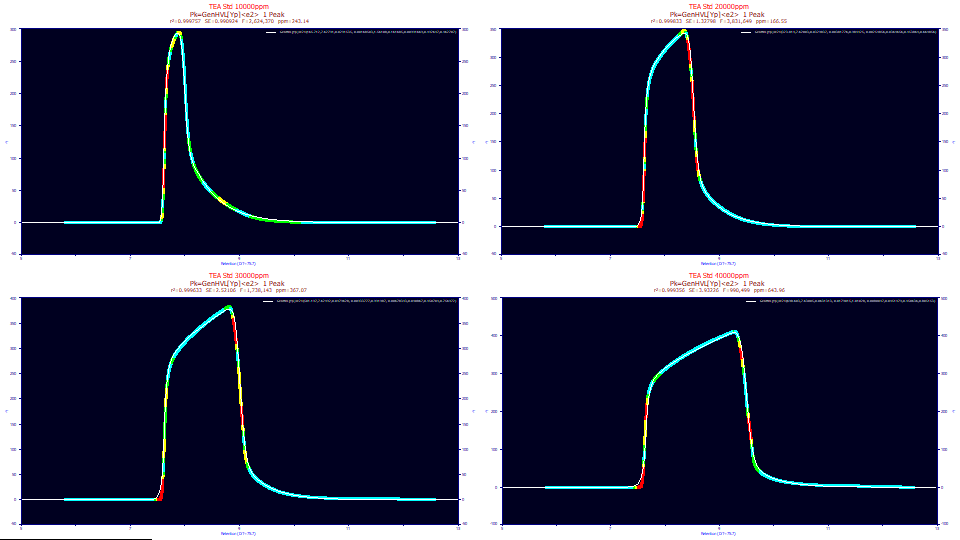
While the fits are quite good, given the vastly distorted shapes, the errors of 243, 166, 367, 643 ppm are well removed from the sub-50 ppm typically seen on analytical shapes.
"TEA�Std�10000ppm"
Fitted�Parameters
r2�Coef�Det�� DF�Adj�r2���� Fit�Std�Err�� F-value������ ppm�uVar
0.99975686��� 0.99975643��� 0.99092398��� 2,624,370���� 243.142042
�Peak Type���������� ������a0���� ������a1���� ������a2���� ������a3���� ������a4���� ������a5���� ������a6���� ������a7���� ������a8��
����1�� GenHVL[Yp]<e2>�� 165.712367�� 7.62790616�� 0.02915358�� -0.0016850�� 1.56108587�� 0.16168679�� 0.49264681�� 0.00991622��0.53729199��
Deconvolved�Moments
�Peak�� Type�������� ���Area����� ���Mean����� ��StdDev���� �Skewness��� �Kurtosis��� �Amplitude�� ���Center�����
����1�� HVL��������� 165.712367�� 7.71770294�� 0.04489006�� -0.7019512�� 2.91901600�� 1649.72479�� 7.75823777��
Advanced�Area�Analysis
�Peak�� Type������������ ����Area���� ��%�Area���� �ApexAsym��� �NonOverlap1 ��%�PkArea�� �NonOverlap2 ��%�PkArea��
����1�� GenHVL[Yp]<e2>�� 165.706546�� 100.000000�� 1.47867118�� 88.3333028�� 53.3070690�� 58.3726815�� 35.2265393��
"TEA�Std�20000ppm"
Fitted�Parameters
r2�Coef�Det�� DF�Adj�r2���� Fit�Std�Err�� F-value������ ppm�uVar
0.99983345��� 0.99983316��� 1.32798346��� 3,831,649���� 166.545420
�Peak Type���������� ������a0���� ������a1���� ������a2���� ������a3���� ������a4���� ������a5���� ������a6���� ������a7���� ������a8��
����1�� GenHVL[Yp]<e2>�� 323.814430�� 7.62002945�� 0.03298375�� -0.0038178�� 0.98442511�� -0.0025486�� 0.45386384�� 0.03646563��0.33514355��
Deconvolved�Moments
�Peak�� Type�������� ���Area����� ���Mean����� ��StdDev���� �Skewness��� �Kurtosis��� �Amplitude�� ���Center�����
����1�� HVL��������� 323.814430�� 7.76191624�� 0.06365485�� -0.6934033�� 2.79079270�� 2333.81036�� 7.82965650��
Advanced�Area�Analysis
�Peak�� Type������������ ����Area���� ��%�Area���� �ApexAsym��� �NonOverlap1 ��%�PkArea�� �NonOverlap2 ��%�PkArea��
����1�� GenHVL[Yp]<e2>�� 323.807068�� 100.000000�� 0.46231684�� 229.137593�� 70.7636168�� 54.5986678�� 16.8614812��
"TEA�Std�30000ppm"
Fitted�Parameters
r2�Coef�Det�� DF�Adj�r2���� Fit�Std�Err�� F-value������ ppm�uVar
0.99963293��� 0.99963229��� 2.52106273��� 1,738,143���� 367.067242
�Peak Type���������� ������a0���� ������a1���� ������a2���� ������a3���� ������a4���� ������a5���� ������a6���� ������a7���� ������a8��
����1�� GenHVL[Yp]<e2>�� 501.196639�� 7.62492405�� 0.04796292�� -0.0093378�� 0.99198708�� -0.0067834�� 0.45070353�� 0.04086680��0.24302761��
Deconvolved�Moments
�Peak�� Type�������� ���Area����� ���Mean����� ��StdDev���� �Skewness��� �Kurtosis��� �Amplitude�� ���Center�����
����1�� HVL��������� 501.196639�� 7.85002070�� 0.09845306�� -0.6871550�� 2.75980363�� 2346.76645�� 7.95814291��
Advanced�Area�Analysis
�Peak�� Type������������ ����Area���� ��%�Area���� �ApexAsym��� �NonOverlap1 ��%�PkArea�� �NonOverlap2 ��%�PkArea��
����1�� GenHVL[Yp]<e2>�� 501.184448�� 100.000000�� 0.29514841�� 362.272018�� 72.2831722�� 50.2737025�� 10.0309782��
"TEA�Std�40000ppm"
Fitted�Parameters
r2�Coef�Det�� DF�Adj�r2���� Fit�Std�Err�� F-value������ ppm�uVar
0.99935605��� 0.99935491��� 3.93225491��� 990,502������ 643.954884
�Peak Type���������� ������a0���� ������a1���� ������a2���� ������a3���� ������a4���� ������a5���� ������a6���� ������a7���� ������a8��
����1�� GenHVL[Yp]<e2>�� 698.602806�� 7.63006608�� 0.06314201�� -0.0179053�� 1.01030860�� -0.0080049�� 0.45060925�� 0.04512322�0.19485141��
Deconvolved�Moments
�Peak�� Type�������� ���Area����� ���Mean����� ��StdDev���� �Skewness��� �Kurtosis��� �Amplitude�� ���Center�����
����1�� HVL��������� 698.602806�� 7.94467842�� 0.13539268�� -0.6823806�� 2.73911603�� 2385.63939�� 8.09634866��
Advanced�Area�Analysis
�Peak�� Type������������ ����Area���� ��%�Area���� �ApexAsym��� �NonOverlap1 ��%�PkArea�� �NonOverlap2 ��%�PkArea��
����1�� GenHVL[Yp]<e2>�� 698.568754�� 100.000000�� 0.22800778�� 509.408942�� 72.9218046�� 48.8806517�� 6.99725709��
The a1 locations are nearly identical, despite the immensely different shapes. The a4 power of decay value, is 1.56 for the least overloaded shape (1% concentration). The other three (2,3,4% concentration) are all very close to the exponential 1.0 power of tailing. The a5 asymmetry converges to very close to a symmetric zero-distortion density as the overload envelope fully forms. The a6 slow exponential in the IRF is nearly constant across the four samples and far wider than the highest distortions observed in analytic peaks. The a8 area fraction of this higher width exponential component in the IRF dramatically decreases with increasing overload. There is a great deal of information in a preparative peak fit, and we will now cover those in more detail.
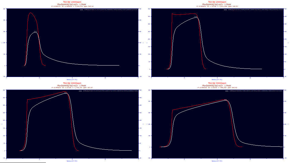
The white peaks are those registered by the instrument. The red peaks are the peaks you would see if there existed no system/instrumental distortion. These are the fitted peaks, the GenHVL[Yp] with the <e2> IRF removed. Although the IRF attenuates the peak and significantly smears out the shape, especially with respect to a broad tailing, note that the overall shape of the overload envelope comes from the twice-generalized chromatographic model, not from the IRF.
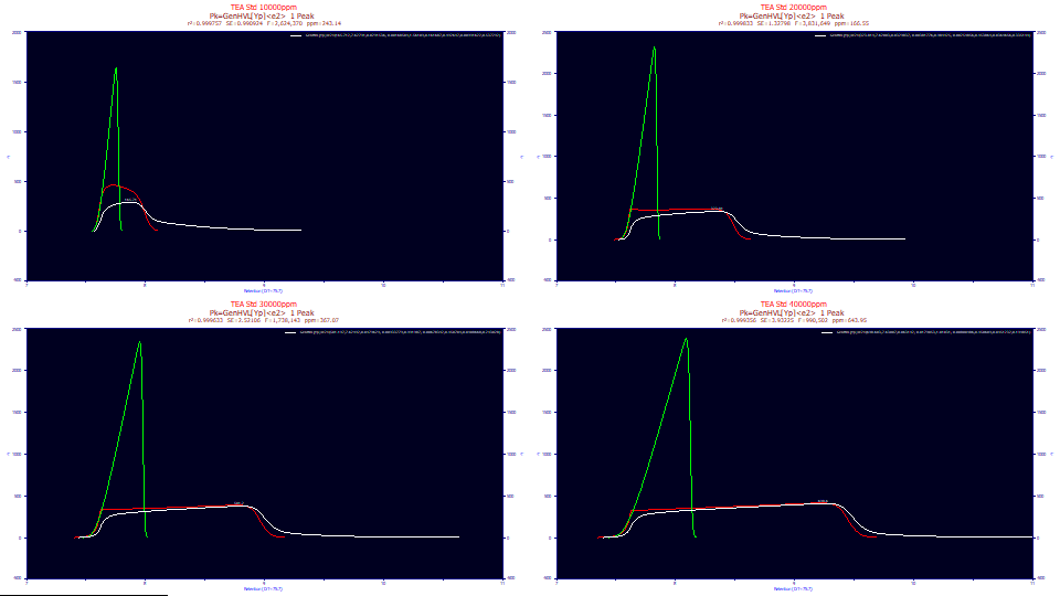
If we use just the pure HVL parameters from the twice-generalized HVL model, we see the green peaks, the pure HVL without the influence of the ZDD's third and fourth moment parameters. This is the pure chromatographic peak you would expect to see if the the column/detector were immune to overload and there existed no higher moment nonidealities. As you will note, the green deconvolved HVL is sharply fronted, even to the point of almost having a right-triangular shape. Even peaks with very little a3 chromatographic distortion at analytical concentrations will have that small measure of fronting or tailing vastly amplified by concentration. The deconvolved preparatory peaks, of very high concentration, as in the green HVL's above, should either be strongly fronted or strongly tailed, depending on the sign of a3. One of the key benefits of preparative shape modeling is the recovery of the peak that would have been observed if the chromatographic instrument had unlimited capacity.
There is a fair argument for seeking a refinement of this workhorse twice-generalized model for fitting preparative shapes. Despite the IRF decreasing with overload (confirmed with a8, the area fraction of the IRF's very large width component), the error of fit actually increases, suggesting the lack of fit rests with the core model, not the accounting of the IRF. While we would not expect such massively distorted shapes to fit as well as analytic peak shapes, we would prefer to see sub-100 ppm fit errors, if possible.
The dilation in the ZDD rests with parameter a4, the power of decay. It fit to 1.56 for the partial overload shape, and very close to 1.0 for all three of the full envelope (a plateau between the rise and decay) data sets. A 2.0 power of decay is that of the Gaussian, 1.0 that of an exponential. Note that a4 maps a constant dilation of 1.0 once a full envelope has formed, and varies between 2 and 1 as the overload increases. The a4 dilation maps the overload shape, but only until a full envelope has formed. The a4 parameter can thus be seen as mapping the extent to which this envelope has formed.
The a7 high width exponential in the IRF fits to a constant .45 in the three full envelope overload data sets. This is about ten times the highest width observed for this instrument with analytic peaks. Since it was apparent just from visual inspection that the amount of this IRF tailing was itself saturated (decreasing proportional to peak area), the a8 area fraction of this largest width component also measures the overload, albeit in a very different way. Unlike analytic peaks where the IRF is somewhat constant, it is far from such in overload shapes. With respect to a7, the smaller of the two exponential widths, we must refer to the analytic <e2> IRF of [tau 1=.007, tau 2=.044, areafrac1=.62]. The a7 parameter certainly fit to the higher analytic width in the three full envelope fits. In case you were wondering if the two exponentials are needed, fits with the GenHVL[Yp]<e> model, a single exponential IRF, were terrible: 2376 ppm to 13140 ppm. As we have shared throughout these white papers, fitting the IRF is essential in high accuracy chromatographic modeling, and overload shapes have massive IRFs.
We will look at a0-a3 parameter values at the four concentrations:
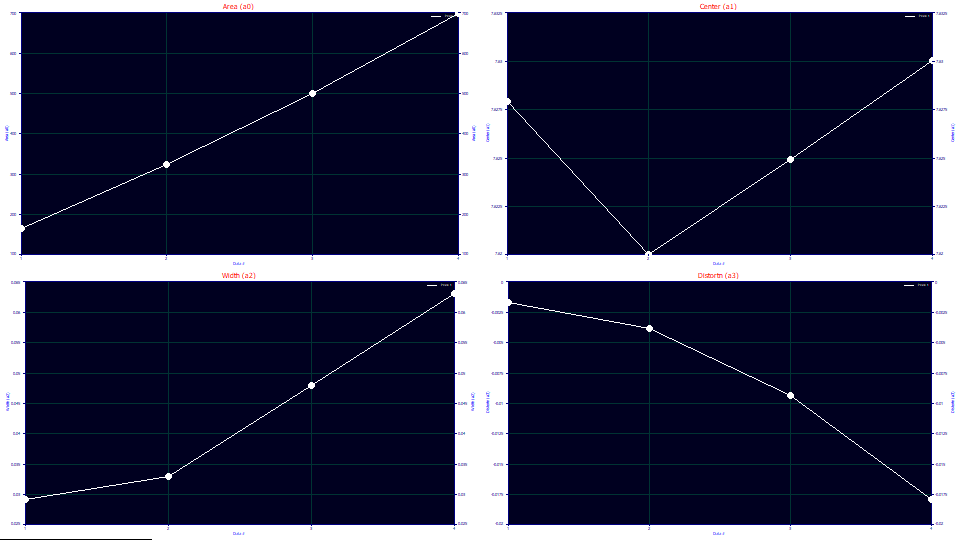
In the first graph, the a0 areas track concentration almost linearly.
One of the suggestions this model is theoretically sound for overload peaks is that the a1 locations are almost perfectly identical for the four vastly different overload shapes (the second graph scales a1 from 7.62 to 7.63).
The a2 widths increase with overload, and linearly once a full envelope is present. For this model, a2 is the SD width of the underlying Gaussian.
The a3 chromatographic shape, strongly fronted, becomes more negative (more fronted) with concentration, another suggestion the model is tracking the overload well. Unlike the linearity of a3 with concentration observed with analytic peaks, the distortion increases with a power greater than 1. If a 0,0 point is inserted into the data (0 chromatographic distortion at 0 concentration), the data in this plot fit to a power of 2.15. In a full accuracy analytic fit, it is our experience that a3 is linear with concentration. Since these fits still have a measure of error, however, we cannot automatically assume overload produces a disproportionate measure of chromatographic distortion.
If the initial rise of the fits are zoomed-in, for the second through fourth data set, there is a significant error in the initial rise. It increases with concentration, and corresponds with the poorer goodness of fit:
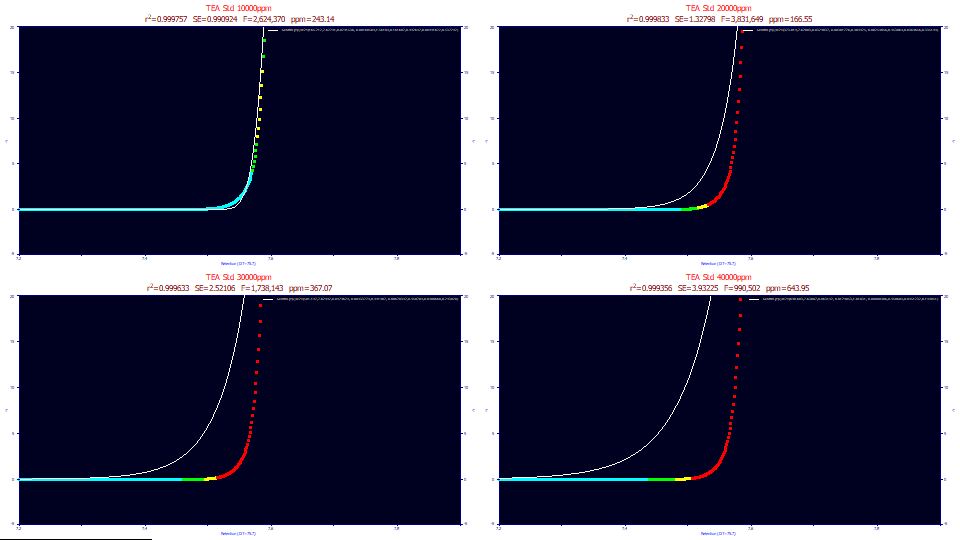
This is the precisely the issue the two-width GenHVL[Yp2] model is designed to solve.
Fitting the Two-Width GenHVL[Yp2]<e2>
In the GenHVL[Yp2] peak the rise of the peak is independently fitted. The addition of an additional rise width parameter (expressed as a width asymmetry, a right-side width divided by a left-side width) changes the basic model from a six-parameter to a seven-parameter one. With a three parameter <e2> IRF added, we fit ten total parameters instead of nine.
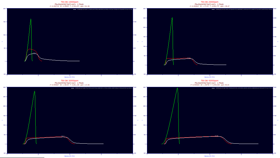
We now better model the nuances in the rise of the overload shape. In the GenHVL[Yp]<e2> fits, we had an average F-statistic of 2.3 million and 355 ppm unaccounted variance across the four fits. In these GenHVL[Yp2]<e2> fits, this one additional parameter resulted in an average F-statistic of 4.3 million and 147.1 ppm unaccounted variance. This one parameter dramatically increased the power and efficacy of the fitting.
We see the about the same red IRF-removed overload shapes, and similar green deconvolved HVL peaks which now increase in amplitude as well as in width with concentration. Intuitively, we would expect at least some increase in amplitude of the deconvolved HVL with the increasing concentration. With the better fitting of the narrow rise of the overload shape, the ZDD is changed in shape, and this is translating differently in the common chromatographic distortion mathematics.
Analyzing the GenHVL[Yp2]<e2>
TEA�Std�10000ppm"
Fitted�Parameters
r2�Coef�Det�� DF�Adj�r2���� Fit�Std�Err�� F-value������ ppm�uVar
0.99975802��� 0.99975754��� 0.98866004��� 2,343,472���� 241.984910
�Peak Type������������� ������a0���� ������a1���� ������a2���� ������a3���� ������a4���� ������a5���� ������a6���� ������a7�����������a8�������a9����
����1�� GenHVL[Yp2]<e2>�� 165.699591�� 7.63050683�� 0.02978956�� -0.0017667�� 0.95382969�� 1.59973390�� 0.17562770�� 0.49175606��0.00753349��0.53574798��
Deconvolved�Moments
�Peak�� Type��������� ���Area����� ���Mean����� ��StdDev���� �Skewness��� �Kurtosis��� �Amplitude�� ���Center�����
����1�� HVL���������� 165.699591�� 7.72274368�� 0.04594607�� -0.7020460�� 2.91801540�� 1612.09703�� 7.76429890��
Advanced�Area�Analysis
�Peak�� Type������������� ����Area���� ��%�Area���� �ApexAsym��� �NonOverlap1 ��%�PkArea�� �NonOverlap2 ��%�PkArea��
����1�� GenHVL[Yp2]<e2>�� 165.693877�� 100.000000�� 1.48240727�� 86.6831801�� 52.3152586�� 57.8075050�� 34.8881360��
"TEA�Std�20000ppm"
Fitted�Parameters
r2�Coef�Det�� DF�Adj�r2���� Fit�Std�Err�� F-value������ ppm�uVar
0.99986153��� 0.99986126��� 1.21101447��� 4,095,737���� 138.471680
�Peak Type������������� ������a0���� ������a1���� ������a2���� ������a3���� ������a4���� ������a5���� ������a6���� ������a7�����������a8�������a9����
����1�� GenHVL[Yp2]<e2>�� 323.663348�� 7.61759861�� 0.03119390�� -0.0032068�� 1.36941334�� 0.99724048�� -0.0023158�� 0.46311223��0.03531645��0.32664782��
Deconvolved�Moments
�Peak�� Type��������� ���Area����� ���Mean����� ��StdDev���� �Skewness��� �Kurtosis��� �Amplitude�� ���Center�����
����1�� HVL���������� 323.663348�� 7.74673995�� 0.05864179�� -0.6957895�� 2.80457939�� 2526.30873�� 7.80823084��
Advanced�Area�Analysis
�Peak�� Type������������� ����Area���� ��%�Area���� �ApexAsym��� �NonOverlap1 ��%�PkArea�� �NonOverlap2 ��%�PkArea��
����1�� GenHVL[Yp2]<e2>�� 323.654534�� 100.000000�� 0.47529531�� 237.337848�� 73.3306111�� 53.8176966�� 16.6281300��
"TEA�Std�30000ppm"
Fitted�Parameters
r2�Coef�Det�� DF�Adj�r2���� Fit�Std�Err�� F-value������ ppm�uVar
0.99988660��� 0.99988637��� 1.40142174��� 5,001,186���� 113.404675
�Peak Type������������� ������a0���� ������a1���� ������a2���� ������a3���� ������a4���� ������a5���� ������a6���� ������a7�����������a8�������a9����
����1�� GenHVL[Yp2]<e2>�� 500.746011�� 7.61641433�� 0.04293464�� -0.0062967�� 2.47162746�� 1.02681407�� -0.0073440�� 0.51548379��0.03705191��0.20461323��
Deconvolved�Moments
�Peak�� Type��������� ���Area����� ���Mean����� ��StdDev���� �Skewness��� �Kurtosis��� �Amplitude�� ���Center�����
����1�� HVL���������� 500.746011�� 7.79795859�� 0.08191696�� -0.6944676�� 2.79675726�� 2801.67097�� 7.88458338��
Advanced�Area�Analysis
�Peak�� Type������������� ����Area���� ��%�Area���� �ApexAsym��� �NonOverlap1 ��%�PkArea�� �NonOverlap2 ��%�PkArea��
����1�� GenHVL[Yp2]<e2>�� 500.709732�� 100.000000�� 0.32286923�� 391.254383�� 78.1399597�� 47.1495800�� 9.41654954��
"TEA�Std�40000ppm"
Fitted�Parameters
r2�Coef�Det�� DF�Adj�r2���� Fit�Std�Err�� F-value������ ppm�uVar
0.99990538��� 0.99990519��� 1.50749340��� 5,993,965���� 94.6232557
�Peak Type������������� ������a0���� ������a1���� ������a2���� ������a3���� ������a4���� ������a5���� ������a6���� ������a7�����������a8�������a9����
����1�� GenHVL[Yp2]<e2>�� 697.884878�� 7.61608517�� 0.05551610�� -0.0110583�� 3.66288634�� 1.06518094�� -0.0085090�� 0.61958737��0.03773216��0.12932068��
Deconvolved�Moments
�Peak�� Type��������� ���Area����� ���Mean����� ��StdDev���� �Skewness��� �Kurtosis��� �Amplitude�� ���Center�����
����1�� HVL���������� 697.884878�� 7.85788217�� 0.10811585�� -0.6925349�� 2.78610988�� 2963.63704�� 7.97350246��
Advanced�Area�Analysis
�Peak�� Type������������� ����Area���� ��%�Area���� �ApexAsym��� �NonOverlap1 ��%�PkArea�� �NonOverlap2 ��%�PkArea��
����1�� GenHVL[Yp2]<e2>�� 697.677056�� 100.000000�� 0.26052019�� 559.392444�� 80.1792806�� 42.6207683�� 6.10895369��
The most significant item is that the goodness of fit improves as the concentration and envelope increase, and as the high width IRF component fraction diminishes in the overall IRF. We note that the GenHVL[Yp2] did not substantially improve the fit of this first data set with its partial overload envelope. Note that an a4 width asymmetry of 1.0 is an equal width to the left and right of the apex, reducing to the GenHVL[Yp] model. On this first data set, a4 fit to 0.953 on this first peak, close to equal widths. The
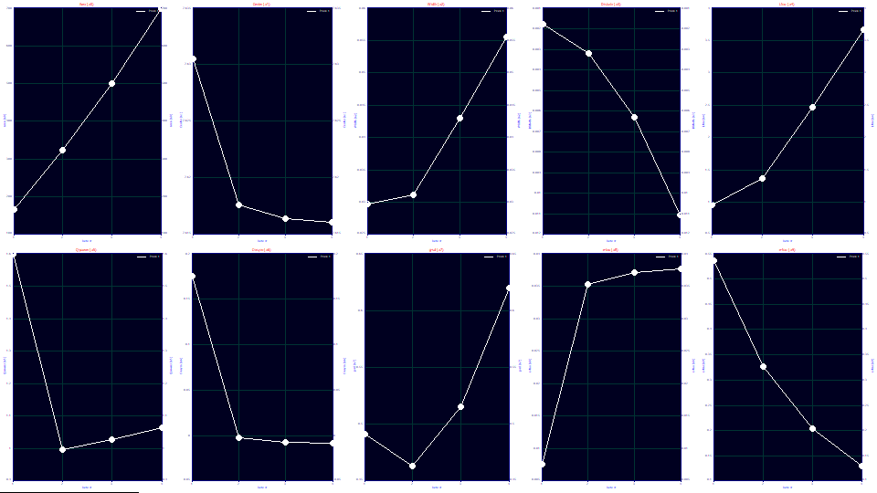
In the above plots, we see all ten parameters, from a0 through a9 lotted against the concentration of overload. As with the single width overload model, a0 tracks concentration, and a1, the deconvolved Gaussian mean, is close to a constant for all four overload shapes (the second graph scales a1 from 7.615-7.635). The a2 deconvolved Gaussian SD in the third graph increases with concentration and overload, again as was observed with the GenHVL[Yp] fits. The single width GenHVL[Yp] and two-width GenHVL[Yp2] models differ little in a2 values until the overload becomes extreme. The a3 chromatographic distortion in the fourth graph, describing the fronting, increases with concentration, although not linearly as if often the case at analytic concentrations. With this GenHVL[Yp2] model, the nonlinearity between a3 and concentration is such that the data fit to a power of 1.7 as compared to 2.15, not the 1.0 linearity we perhaps wished to see, but an improvement.
The new parameter a4 is a width-based asymmetry, the right side width divided by the left side width. This parameter, shown in the fifth graph, also strongly tracks the overload, linearly with a full envelope. For the last of the data sets, the a4=3.66 width asymmetry means that the right side of the peak is computed using a width of a2*a4/(1+a4) or .0436 and the left side of peak is computed using a width of a2/(1+a4) or .0119. The right side width of the [Yp2] ZDD density is 3.66x larger than the left side.
The a5 ZDD power of decay in the sixth graph remains close to 1.0 for the full overload envelope data sets, and at 1.60, we see close to the GenHVL[Yp] 1.56 power of decay value for the first data set with the partial envelope. In both the GenHVL[Yp] and GenHVL[Yp2] fits, the power of decay increased slightly with concentration for the full envelope fits. With the separate rise and decay widths, this deviation from 1.0 is greater with the GenHVL[Yp2] model.
The a6 ZDD asymmetry in the seventh graph shows the first partial overload data set fitting to a strong right-skewed asymmetry. The three full overload sets fit to slightly negative values as did the GenHVL[Yp] fits.
The a7, a8, a9 parameters describing the <e2> IRF are in the last three graphs. Unlike the GenHVL[Yp] fits, the two-width fits produce the more extended a7 widths we saw in the original contours of the tails in the data. This a7 exponential component which produces the huge tailing now increases with concentration. The amount of the component a9 diminishes with concentration as did the single-width fits.
The numeric results, shown above, furnish the moments of the deconvolved HVL peaks as well as an advanced area analysis which estimates the measure of non-overlap between the green HVL and the red curve absent the IRF, and this red curve relative to the peak as registered by the instrument.
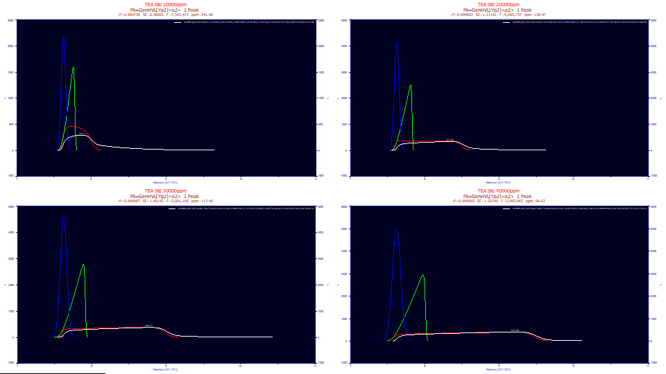
We now add a last level of deconvolution. The blue curves above plot the deconvolved Gaussian, the peak this two-width overload model predicts if there was no IRF, no higher moment nonidealities, and no concentration-dependent a3 chromatographic distortion.
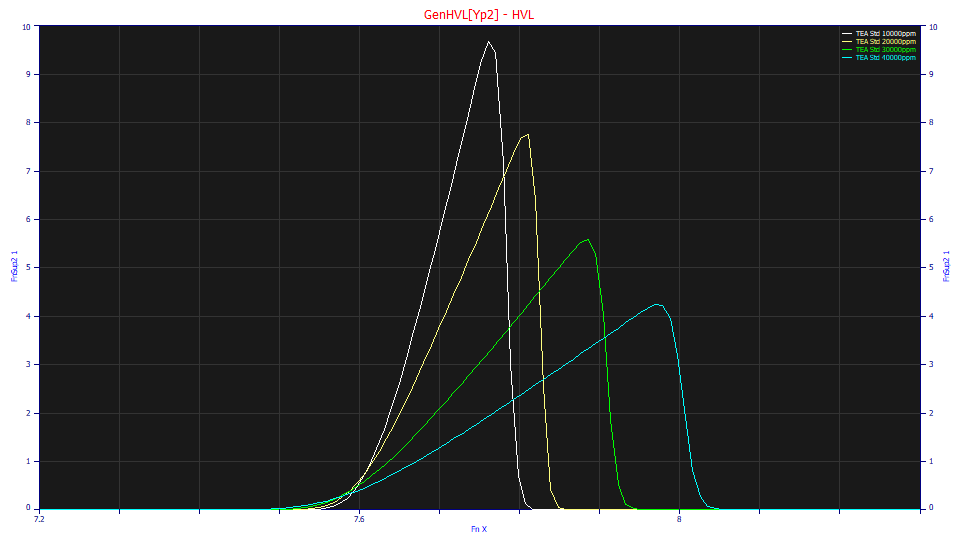
The deconvolved HVLs are shown in the above plot with normalized areas. As we observed in the fitted values, the a3 chromatographic distortion, the fronting, continues to increase with concentration, but a2, the Gaussian width also increases with concentration.
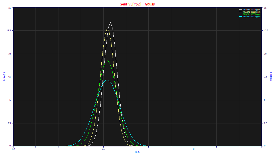
The deconvolved Gaussians remove the chromatographic distortion of the HVL, but the broadening with concentration is also evident. Note that the three full-envelope peaks have almost identical Gaussian locations and differ only in this broadening. Only the first shape with the partial overload, which did not fit quite as well, shows any locational variation.
Concentration and a2
Since the overload model fits suggest that there is this broadening with very high levels of concentration in the deconvolved peaks, we conclude this white paper with a discussion of whether or not this premise has any support at analytical concentrations where no overload occurs.
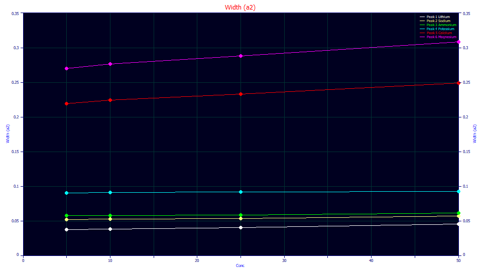
In fitting analytic peaks, we have indeed observed an increase in a2 with an increase in analytic concentrations. The above plot is for GenHVL<ge> fits of the cation data that was used in the first of these white papers. The increase is a2 appears to track the magnitude of the a3 distortion. The a3 distortion is greatest in magnitude in the Ca+ (red) and Mg+ (magenta), the strongly tailed peaks, and those do show an increase in a2 with concentration. The K+ peaks (cyan) have very little a3 distortion, and they are close to constant in a2 across concentration. The Li+ peaks (white) have the strongest fronting, and also have the highest increase in a2 with concentration for the three different species that produce fronted peaks.
Higher Moment Chromatographic Models and IRFs
In these four white papers we have shown that higher moment models, based on the longstanding established science of the Haarhoff-VanderLinde and Wade-Thomas models, in conjunction with real-world IRF fitting, can result in close to zero error in fitting a wide variety of chromatographic shapes, including two of the most difficult challenges in chromatographic modeling, gradient HPLC and preparative shapes. The science of the core models has been in place for decades and in our experience it is complete with respect to the peak fitting of chromatographic shapes, sufficient for a rigorous implementation in both production and analytical environments. The additions we describe in these white papers include the addition of higher moment adjustments to these core chemical engineering models, this based on well-established advances in the statistical sciences, and the addition of IRF convolution and deconvolution, this drawn from the well-established digital signal processing sciences.