PeakLab v2 Documentation Contents R2N Software Home R2N Software Support
Common Chromatographic Distortion Model
Equivalence
The Wade-Thomas NLC model, while derived for affinity chromatography, and the HVL, designed primarily for GC peak shapes, but widely used in many forms of chromatography, employ common distortion mathematics which can result in identical distorted shapes in chromatographic peak fitting. This discovery of equivalence, that of a common distortion model for chromatographic peak models, is central to the modeling technology in PeakLab.
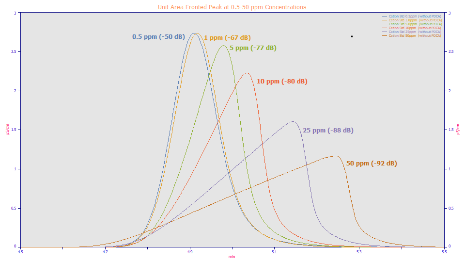
Nonlinear Chromatography and Fronted Distortions

In the HVL and Wade-Thomas NLC models, a peak dramatically changes shape with concentration. In the above plot with a unit area normalization for all peaks, concentrations are shown for a range to two orders of magnitude. A intrinsically fronted peak will be fronted (have a negative a3 distortion value) at all concentrations, and further, we have found a3 to be linear with concentration when the instrumental effects are accounted. That is, the greater the magnitude of the -a3 value, the greater the fronting. In the above plot, we show the approximate S/N thresholds. The higher concentrations produce significantly better S/N, but the fronting also sharply increases. Note also that the two samples at the lowest concentrations appear tailed, even though the peaks are intrinsically fronted in the chromatographic separation. The extracolumn or instrumental effects produce the observed tailing and are more discernible than the intrinsic fronting.
Nonlinear Chromatography and Tailed Distortions
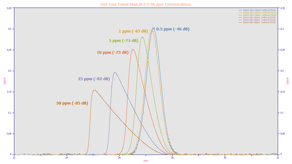
The same concentration dependency occurs with intrinsically tailed peaks. Again, the plot is made with a unit area normalization for all of the tailed peaks, and the concentrations are again shown for a range to two orders of magnitude. A intrinsically tailed peak will be tailed (have a positive a3 distortion value) at all concentrations. And here as well we found a3 to be linear with concentration when all extracolumn effects are properly fitted. The greater the a3 value, the greater the tailing. For this example, the S/N thresholds are somewhat lower. The higher concentrations produce significantly better S/N, but the tailing also increases. Note also that the two samples at the lowest concentrations appear Gaussian, even though the peaks are intrinsically tailed. The extracolumn or instrumental tailing combines with the intrinsic tailing and both are little visible when the broadening is high at long elution times.
It is the concentration dependency shown above that is treated identically in the distortion mathematics of the HVL and Wade-Thomas NLC models. The models use a different parameterization, but when the models are templated and each is given a common zero-concentration (infinite dilution) density assumption, the distortion mathematics produce identical shapes.
The Generalized HVL and NLC Model Templates
In the ZDD concepts topic, we derived the HVL generalized template:
The HVL model is reproduced by substituting the Gaussian or normal PDF and CDF for the Density and Cumulative in the formula.
To simplify matters, we will revise the NLC Template to use the cumulative of the density rather than the reverse cumulative or complement of the CDF. After simplification, the NLC template looks surprisingly close to the HVL template. The only difference is that a3 is scaled by a1/a2 in the HVL template.
The NLC model is reproduced by substituting the Giddings PDF and CDF for the Density and Cumulative in the formula.
For both templates the parameters have the same correspondence with moments:
a0 = area of the overall model
a1 = the center value used in the density and cumulatives
a2 = the width value used in the density and cumulatives
a3 = the HVL or NLC chromatographic distortion parameter (fronted for a3<0, tailed for a3>0)
Density = PDF for the specified ZDD (zero distortion density), area=1
Cumulative = CDF for the specified ZDD, magnitude=1
RevCumulative = CDF complement for the ZDD, magnitude=1
Note that a1 and a2 derive their meaning in the Density and Cumulative elements. The HVL Template's a1/a2 adjustment of the distortion linearizes the a3 distortion with concentration for a Gaussian-based zero-distortion density. The NLC Template, when using a kinetic peak such as the Giddings, requires no adjustment for an a3 distortion that is linear with concentration.
Generalized HVL and Generalized NLC Template Conversion
Conversion between the templates is straightforward. The only difference is this center/width scale factor:
A Common Distortion Operator for Chromatographic Data
PeakLab's generalized models use statistical generalizations which reduce to the normal density through one or two levels of generalization. Since there exist a wealth of well-researched statistical generalizations of densities, and even the simplest of the kinetic models using this a3 common distortion (the NLC with the Giddings ZDD) is at the bounds of computational viability, we use the HVL Template and statistical generalizations to manage the third and fourth moments of chromatographic peaks. We then use an equivalence relationship for the generalized NLC models.
When the GenHVL model fits perfect NLC data, its a3 distortion values will be twice that of the NLC a3 distortion. In order to have a truly common distortion operator, we adjusted the GenNLC a3 distortion to exactly match the GenHVL a3 distortion. You will see the same a3 distortion value whether you are looking at a chromatographic peak as a scaled diffusion-type model (GenHVL), or as a first order kinetics peak (GenNLC).
The GenNLC's a3 will thus be twice the value of the NLC's a3 and identical to the GenHVL's a3 distortion value.
The different aspects of the equivalence between the diffusion-type GenHVL and kinetic-type GenNLC models will become clearer when using the Equivalent Parameters section of the Numeric Summary when fitting either a GenHVL or GenNLC model.
The NLC and HVL a3 Distortion
Even though the GenHVL and GenNLC, the generalized models using a generalized normal can each fit both the HVL and NLC shapes, there are issues which must be considered when peaks eluting at different times share this a3 common distortion parameter. This is not normally done, but may be necessary when fitting a small band of highly overlapped peaks. It will definitely be necessary when there are hidden peaks.
This choice to implement statistical ZDDs to model the kinetics impacts the behavior of a3 across elution time. To fully understand this common chromatographic distortion, we will create a sequence of HVL and NLC peaks.
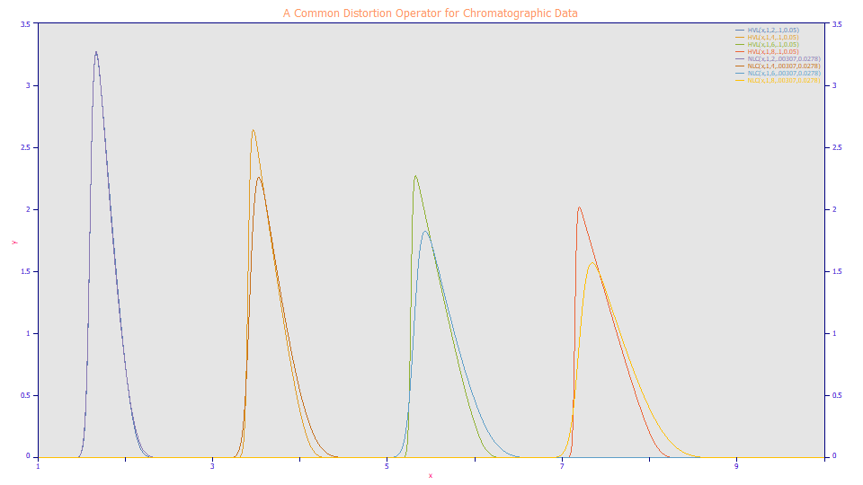
The NLC and HVL models cannot replicate the same chromatographic shapes. The NLC assumes a Giddings ZDD, a kinetic peak which broadens with location at constant a2 values, even with no a3 chromatographic distortion. The HVL assumes a Gaussian ZDD, a scaled statistical peak where a given a2 produces an identical width independent of the a1 location. The two models can, however, be parameterized to be somewhat close in shape. That was done for the HVL and NLC peaks at x=2 in the plot above. There are four HVL peaks sharing a common a2 and a3 and varying only by a1 location. Similarly, there are four NLC peaks with their own common a2 and a3 which also vary only by location.
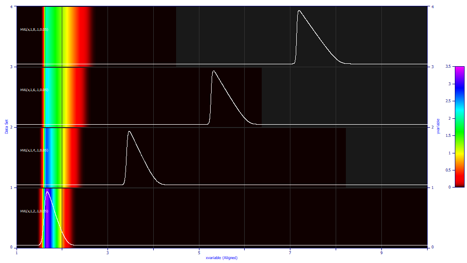
These are the four HVL peaks with alignment of contour unit area maxima. With the maxima aligned, the left side of the peak diminishes and the right side increases with elution time for a constant a3:
Fitted�Parameters
r2�Coef�Det�� DF�Adj�r2���� Fit�Std�Err�� F-value������ ppm�uVar
1.00000000��� 1.00000000��� 2.3702e-7���� 3.9922e+14��� 1.5631e-6�
�Peak�� Type���� ������a0���� ������a1���� ������a2���� ������a3���� ������a4����
����1�� GenHVL�� 0.24999995�� 1.99999991�� 0.09999959�� 0.04999978�� -1.037e-6���
����2�� GenHVL�� 0.24999993�� 3.99999927�� 0.09999938�� 0.04999958�� -1.037e-6���
����3�� GenHVL�� 0.24999993�� 5.99999864�� 0.09999923�� 0.04999944�� -1.037e-6���
����4�� GenHVL�� 0.24999992�� 7.99999801�� 0.09999911�� 0.04999934�� -1.037e-6���
Equivalent�Parameters
�Peak�� Type���� ������a0���� ������a1���� ������a2���� ������a3���� ������a4����
����1�� GenNLC�� 0.24999995�� 1.99999991�� 0.00249998�� 0.04999978�� -2.074e-5���
����2�� GenNLC�� 0.24999993�� 3.99999927�� 0.00124998�� 0.04999958�� -4.148e-5���
����3�� GenNLC�� 0.24999993�� 5.99999864�� 0.00083332�� 0.04999944�� -6.222e-5���
����4�� GenNLC�� 0.24999992�� 7.99999801�� 0.00062499�� 0.04999934�� -8.296e-5���
Measured�Values
�Peak�� Type���� �Amplitude�� ��Center���� ���FWHM����� ��Asym50���� �FW�Base���� ��Asym10����
����1�� GenHVL�� 0.81501472�� 1.67399392�� 0.28966507�� 2.77626888�� 0.59551070�� 3.35218457��
����2�� GenHVL�� 0.66114972�� 3.47107970�� 0.36190008�� 4.71449073�� 0.74367882�� 5.88715727��
����3�� GenHVL�� 0.56839084�� 5.31793008�� 0.42457202�� 6.55985968�� 0.86908116�� 8.30659069��
����4�� GenHVL�� 0.50593121�� 7.19050875�� 0.47964442�� 8.32609035�� 0.97861980�� 10.6382853��
�Peak�� Type���� ���Area����� ��%�Area���� ���Mean����� ��StdDev���� �Skewness��� �Kurtosis���
����1�� GenHVL�� 0.24999995�� 25.0000017�� 1.77533278�� 0.13352289�� 0.67484249�� 3.00086395��
����2�� GenHVL�� 0.24999993�� 25.0000001�� 3.64042572�� 0.17143874�� 0.70204398�� 2.85565192��
����3�� GenHVL�� 0.24999993�� 24.9999993�� 5.53896668�� 0.20256406�� 0.68855370�� 2.76628498��
����4�� GenHVL�� 0.24999992�� 24.9999990�� 7.45453595�� 0.22935499�� 0.67473377�� 2.70919751��
��All�� Total��� 0.99999973�� 100.000000��
If we fit these four HVL peaks to the GenHVL, we see very close to the generated parameters (the model cannot fit the a4 statistical asymmetry perfectly to 0 because of a singularity). Note that the a2 SD of the underlying Gaussian is constant as is the a3 distortion, but the FWHM increases from .290 to .480 and the second moment, as an SD, increases from .133 to .229. The impact on the higher moments is even more pronounced. The half-height asymmetry varies from 2.78 to 8.33. The skewness, the third moment, is strongly tailed and approximately constant, while the kurtosis, the fourth moment, successively drops below the 3.0 of the Gaussian. For the HVL, constant a2 and a3 parameters do not equate to identical peaks shifted only by location. The peaks are becoming much more sharply tailed, as given by the half-height asymmetry, even though the a3 distortion is constant.
Note the Equivalent Parameters section. Had we fit a GenNLC, we would have the same a0, a1, and a3 and the same goodness of fit, but the a2 NLC time constant decreases with elution, not something one would expect to see in practice. Indeed, our experience with the adsorption-desorption kinetics in IC is such that the NLC a2, the Giddings time constant, increases somewhat with elution time. These differences in shape with constant a3 are a consequence of the HVL definition and this a1/a2 scaling. It is unrelated to the asymmetry in the generalized model; in this instance there is none.
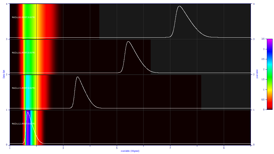
This is a similar plot of the four NLC peaks where the maxima are aligned in the gradient rendering. A constant a2 kinetic width and a3 distortion result in increased breadth on each side of the apex of the peak:
Fitted�Parameters
r2�Coef�Det�� DF�Adj�r2���� Fit�Std�Err�� F-value������ ppm�uVar
1.00000000��� 1.00000000��� 5.062e-16���� 7.3065e+31��� 0.00000000
�Peak�� Type���� ������a0���� ������a1���� ������a2���� ������a3���� ������a4����
����1�� GenNLC�� 0.25000000�� 2.00000000�� 0.00307000�� 0.05560000�� 0.50000000��
����2�� GenNLC�� 0.25000000�� 4.00000000�� 0.00307000�� 0.05560000�� 0.50000000��
����3�� GenNLC�� 0.25000000�� 6.00000000�� 0.00307000�� 0.05560000�� 0.50000000��
����4�� GenNLC�� 0.25000000�� 8.00000000�� 0.00307000�� 0.05560000�� 0.50000000��
Equivalent�Parameters
�Peak�� Type���� ������a0���� ������a1���� ������a2���� ������a3���� ������a4����
����1�� GenHVL�� 0.25000000�� 2.00000000�� 0.11081516�� 0.05560000�� 0.02770379��
����2�� GenHVL�� 0.25000000�� 4.00000000�� 0.15671630�� 0.05560000�� 0.01958954��
����3�� GenHVL�� 0.25000000�� 6.00000000�� 0.19193749�� 0.05560000�� 0.01599479��
����4�� GenHVL�� 0.25000000�� 8.00000000�� 0.22163032�� 0.05560000�� 0.01385190��
Measured�Values
�Peak�� Type���� �Amplitude�� ��Center���� ���FWHM����� ��Asym50���� �FW�Base���� ��Asym10����
����1�� GenNLC�� 0.81906786�� 1.67446070�� 0.28274674�� 2.64603623�� 0.60523050�� 3.33555734��
����2�� GenNLC�� 0.56503247�� 3.53573765�� 0.41206691�� 2.63078712�� 0.87138950�� 3.26829031��
����3�� GenNLC�� 0.45633328�� 5.42928735�� 0.51141649�� 2.62377353�� 1.07568609�� 3.23860912��
����4�� GenNLC�� 0.39263260�� 7.33954438�� 0.59521224�� 2.61951551�� 1.24793836�� 3.22095144��
�Peak�� Type���� ���Area����� ��%�Area���� ���Mean����� ��StdDev���� �Skewness��� �Kurtosis���
����1�� GenNLC�� 0.25000000�� 25.0000000�� 1.77615211�� 0.13719600�� 0.74820263�� 3.20420926��
����2�� GenNLC�� 0.25000000�� 25.0000000�� 3.68040697�� 0.19657134�� 0.72261567�� 3.14585260��
����3�� GenNLC�� 0.25000000�� 25.0000000�� 5.60691585�� 0.24215590�� 0.71136114�� 3.12086748��
����4�� GenNLC�� 0.25000000�� 25.0000000�� 7.54495203�� 0.28059376�� 0.70467533�� 3.10622230��
��All�� Total��� 1.00000000�� 100.000000��
If we fit these four NLC peaks to the GenNLC, we recover the generated parameters to full precision. Note that the a2 kinetic time constant of the underlying Giddings model is constant as is the a3 distortion, and the a4 asymmetry fits to a constant 0.5, the NLC. Here the FWHM increases from .283 to .595 and the second moment, as an SD, increases from .137 to .280. The widening with a constant a2 is appreciably higher. The half-height asymmetry, however, is close to constant for all four of the peaks. The skewness, the third moment is approximately constant, higher than the GenHVL, while the kurtosis, the fourth moment, successively drops but remains above the 3.0 of the Gaussian. For the NLC, constant a2 and a3 parameters equally do not equate to identical peaks shifted only by location.
Note the Equivalent Parameters for the GenHVL. Had we fit the GenHVL to this data, we would have the same a0, a1, and a3. The a2 Gaussian deconvolved SD increases by about a factor of 2 across the peaks, but the a4 asymmetry changes as well, decreasing by a factor of 2. In designing the GenHVL model, we retained the a4 definition as the standard statistical asymmetry of the generalized normal.
Sharing a2 Width, a3 Distortion, and a4 Asymmetry across GenHVL and GenNLC Peaks
The GenHVL and GenNLC models will each fit the theoretical HVL and NLC shapes completely. With the a3 adjusted to be identical across the two models, the only differences rest with the a2 term describing the width, and the a4 term describing the ZDD third moment asymmetry.
The GenHVL and GenNLC are in effect the same model with two different parameterizations of a2 and a4. If fitting only a single peak you will always get the same identical goodness of fit, whether you fit the GenHVL or the GenNLC. The differences arise only when sharing parameters across multiple peaks in an elution.
The a2 and a3 parameters shared only when absolutely necessary, usually when fitting poorly defined overlapping and hidden peaks. On the other hand, the a4 asymmetry is almost always shared, a measure of the ZDD's deviation from theoretical ideality.
You should see the GenHVL as a diffusion theory or statistical peak. The a2 is the deconvolved Gaussian SD and the a4 is the statistical asymmetry of the generalized normal. When there is no asymmetry, a4=0, the peak becomes the pure HVL. When sharing a4, there is a constant asymmetry in the ZDD across all peaks.
You should see the GenNLC as a kinetic theory peak. The a2 is the time constant of the first-order adsorption-desorption of the Giddings model, and the a4 is an asymmetry normalized to the Giddings. When the ZDD is a Giddings shape, the a4 will have a value of 0.5, representing the pure NLC. When there is no no asymmetry, a4=0, the peak becomes the pure HVL. In the GenNLC, sharing the a4 asymmetry is sharing a constant measure of deviation from this a4=0.5 Giddings ideality associated with the NLC.
Since the a4 is the parameter that is typically shared, you are generally choosing between having a constant statistical asymmetry, a constant measure of deviation from the Gaussian in the infinite dilution density used to construct the GenHVL peak, and having a constant measure of the deviation from the Giddings asymmetry in the ZDD which is used to construct the GenNLC peak.
In practice, the differences in goodness of fit between sharing the a4 in a GenHVL model and doing so in a GenNLC model are quite small for most analytic peaks. For example, if the 16 IC cation data sets of the Chromatographic Experiments tutorial are fitted to the GenHVL<ge> model with this shared a4, the average goodness of fit across the sets is 9.92 ppm unaccounted variance. For the GenNLC<ge> model, the average of the 16 different fits is 10.26 ppm error. If instead, we fit the GenHVL<e2> model, we average 10.54 ppm, and for the GenNLC<e2> we average 9.76 ppm. This sufficiently summarizes our experience. The sharing of a4 does have a very small impact, but we cannot confirm either the absolute statistical asymmetry or the Giddings-reference asymmetry as offering better fits. The differences are too small.
Since you can display the parameters for each model in this Equivalent Parameters option in the Numeric Summary, you will always have the diffusion and kinetic widths and the statistical and kinetic asymmetries available in any fit to either model.