PeakLab v1 Documentation Contents AIST Software Home AIST Software Support
HPLC Column Health and Overload (Tutorial)
In this tutorial, we will fit an overload model to peak data from three different columns to see if fitting can distinguish performance issues. In this example, one of the columns was exhibiting poor resolution. This is blood protein data, and the primary amplitude peak is not the target of the analysis. To support a better S/N in the smaller peaks of interest, the concentration is such that this main peak is likely at or near a point where the column is exhibiting some measure of overload. In this tutorial we will use the GenHVL[Yp2] overload model with a <ge> half-Gaussian+exponential IRF to see if we can fit parameters that can serve as indicators of column health.
Importing the Data
![]() Click the Open button, the first button in the program's main toolbar. Select the file ColumnsOverload.pfd
from the program's installed default data directory (\PeakLab\Data).
Click the Open button, the first button in the program's main toolbar. Select the file ColumnsOverload.pfd
from the program's installed default data directory (\PeakLab\Data).
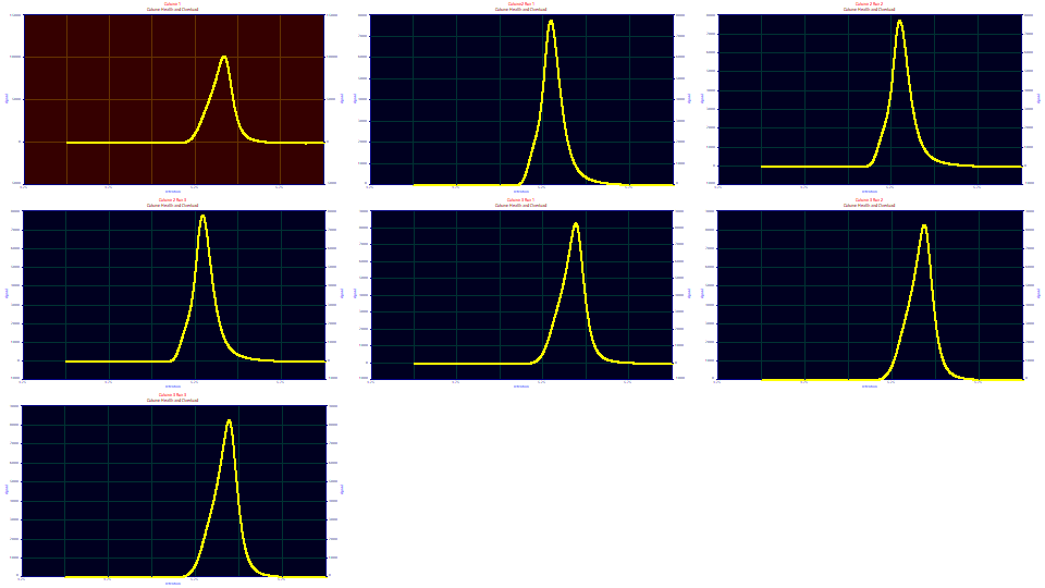
The data has been preprocessed (sectioned and the baseline subtracted) and is ready for fitting. The first data set is from a column deemed to be healthy. The next three peaks are replicates from a column performing poorly. The last three peaks are also replicates, these from a column deemed to have a diminished, but still a reasonably good resolution.
Visualizing the Data
Click the View and Compare Data button. Select Single/Contour, Unit Area, and check Force Zmin=0. Use the mouse in either the upper or lower graph to zoom-in the peaks.
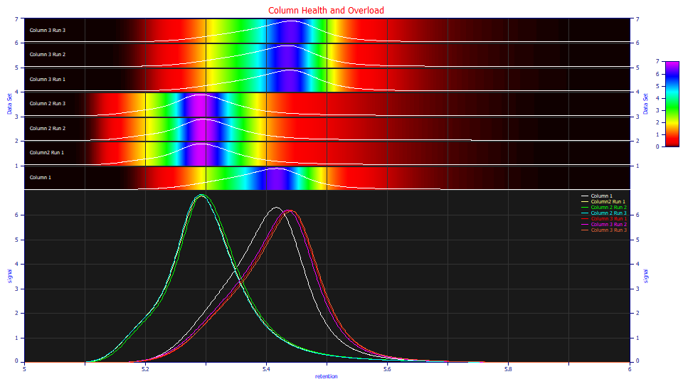
The differences between the three columns are apparent. The replicate runs associated with columns 2 and 3 are good, but do not exactly overlap one another. Those small differences should prove useful in validating the fits. What is clear is that there are very different shapes for the same sample. The poor resolution column 2's principal peak elutes earlier and has an unusual shape, suggestive of two distinct components. These are proteins, and conformations can elute at different points, but here we know column 2 isn't producing a better separation of two components. We begin with the assumption we are looking at just a single component, and the differences in shape are related to sensitivity to overload.
Click OK. Using the mouse, left click the 2nd, 3rd, and 4th graphs. They will be deselected, the background grayed. Once again click the View and Compare Data button and select the Single/Contour plot format. Once again, use the mouse in either the upper or lower graph to zoom-in the peaks.
The column 1 peak elutes slightly earlier. Its rise is also much smoother.
![]() Click the Shift Patches to Align Maxima button in the graph's toolbar. The peaks remain at their
locations, but the gradients are shifted to align with the maximum in data set 1.
Click the Shift Patches to Align Maxima button in the graph's toolbar. The peaks remain at their
locations, but the gradients are shifted to align with the maximum in data set 1.
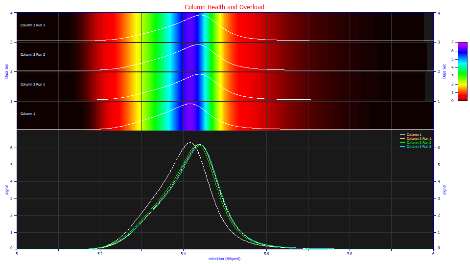
The differences are subtle, but if you use the yellow bands as markers, you see that column 1, when aligned, is narrower and has a flatter larger zone at the maximum. At this point, let us assume we suspect column 1 is healthy, column 3 has a small diminished performance, and column 2 has suffered significant performance degradation.
We are not as concerned with differentiating column 2; when there is a significant difference in the first moment, the center of mass of the elution, we assume we will be able to find a way to model the poor column health parametrically. We are more interested in seeing whether or not we can differentiate columns 1 and 3 parametrically.
Click OK to exit the visualization procedure.
Fitting the GenHVL[Yp2]<ge> Overload Model
In a generalized chromatographic model, the common chromatographic distortion operator is applied to a zero-distortion density (ZDD) to generate the overall peak shape. The ZDDs of a generalized model include adjustments to the third and/or fourth moments of this density which then sees this a3 chromatographic distortion.
For overload conditions, we expect to see a dilation in the fourth moment, a 'fattening' of the tails. The basic twice generalized chromatographic models use a single width specification. If the ZDD happens to be Gaussian, the width used for the left half of the peak, prior to the apex, is the same width as is used for the right half. The [Yp2] ZDD is an exception. It is a speciality model that introduces separate left and right side widths, and this has proven beneficial for high overload preparative shapes. We will use this same modeling technology with these peaks which we assume have retained most of their analytic shapes, the overload only partial.
Since we expect the IRF parameters to be important in any detection of an overload state, or in a poorly performing column where the mass transport or adsorption has changed, we will fit the <ge> IRF, the area-weighted sum of a half-Gaussian and first order exponential response function.
Click the Select All button to re-select all data sets, and then click the Local Maxima Peaks button. Set the selections as follows:
Peak Detection
Set Sm
n(1) to 20
Peak Type
Select Chromatography
in the first dropdown
Select GenHVL[Yp2]<ge> as the model
in the second dropdown
Scan
Set the Amp %
threshold to 1.5 %
Leave Use Baseline Segments unchecked
Be sure Use IRF,ZDD is checked
Vary
Leave width a2
and shape a3 checked, all other unchecked
Click the IRF button. If you made modifications to the IRF defaults prior to this tutorial for your own fitting, please use the Save button to save your IRF values before resetting the defaults. Click the Defaults button. These are based on retention scale averages of modern IC data for each of the IRFs built into the program. Click the Lock button next to the g area fraction in the <ge> IRF. This 5/8 narrow-component, 3/8 wide-component, is a good approximation for many analytic IRFs. For all of these fits, we want the two components of the IRF to be held in same ratio. We do this in part to acknowledge the more difficult fitting of overload shapes. Click OK.
Click the Peak Fit button in the lower left of the dialog to open the fit strategy dialog. Select the Fit with Reduced Data Prefit, 2 Pass, Lock Shared Parameters on Pass 1. Leave the Fit using Sequential Constraints box checked. Click OK. Especially for fitting overload models, you will need this 2-pass option where the main peak parameters are first estimated while the starting estimates for the IRF and/or ZDD are initially held constant.
The fit should require only a few seconds. Click Review Fit.
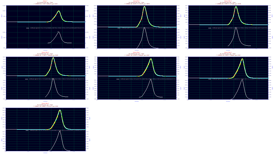
The goodness of fit is poorer for the three column 2 data sets. The goodness of fit for these three column 2 replicates is 95-108 ppm unaccounted variance. For column 3, it is 22.67-24.02. The first column fit to 22.25 ppm. These fits should be good enough for parametric inferences.
Click Numeric. In the Options menu of the Numeric Summary, choose Select Only Fitted Parameters and also check the Chromatography Analysis item.
"Column�1"
Fitted�Parameters
r2�Coef�Det�� DF�Adj�r2���� Fit�Std�Err�� F-value������ ppm�uVar
0.99997775��� 0.99997762��� 11.5799932��� 8,382,213���� 22.2489972
�Peak�� Type������������� ��a0��� �������a1��� �������a2��� �������a3��� �������a4��� �������a5��� ��������a6��� ������a7��� ������a8�����������a9���
����1�� GenHVL[Yp2]<ge>�� 1624.77828�� 5.25253485�� 0.04660691�� -0.0027363�� 1.93658381�� 1.53977982�� -0.2024907�� 0.04585396���0.06755071���0.61132500��
Chromatographic�Analysis
�Peak�� Type������������� ��Nmoment�� ��NGauss��� ��FW�Base���� ��Asym10���� Resolution�� �Retention��
����1�� GenHVL[Yp2]<ge>�� 5062.12600�� 8398.54411�� 0.32228324�� 0.69486775�� ������������ 5.25253485��
"Column2�Run�1"
Fitted�Parameters
r2�Coef�Det�� DF�Adj�r2���� Fit�Std�Err�� F-value������ ppm�uVar
0.99989155��� 0.99989089��� 18.2731032��� 1,719,478���� 108.451330
�Peak�� Type������������� ��a0��� �������a1��� �������a2��� �������a3��� �������a4��� �������a5��� ��������a6��� ������a7��� ������a8�����������a9���
����1�� GenHVL[Yp2]<ge>�� 1143.84988�� 5.25572334�� 0.06524308�� -0.0029166�� 0.22292604�� 1.24299677�� 0.15965577�� 0.03296021���0.08197862���0.61132500��
Chromatographic�Analysis
�Peak�� Type������������� ��Nmoment�� ��NGauss��� ��FW�Base���� ��Asym10���� Resolution�� �Retention��
����1�� GenHVL[Yp2]<ge>�� 4264.92831�� 11255.4421�� 0.32654392�� 1.14048257�� ������������ 5.25572334��
"Column�2�Run�2"
Fitted�Parameters
r2�Coef�Det�� DF�Adj�r2���� Fit�Std�Err�� F-value������ ppm�uVar
0.99989510��� 0.99989446��� 17.8457168��� 1,777,655���� 104.902463
�Peak�� Type������������� ��a0��� �������a1��� �������a2��� �������a3��� �������a4��� �������a5��� ��������a6��� ������a7��� ������a8�����������a9���
����1�� GenHVL[Yp2]<ge>�� 1129.70255�� 5.25972271�� 0.06366625�� -0.0027587�� 0.22890857�� 1.24625648�� 0.15874912�� 0.03268072���0.08175537���0.61132500��
Chromatographic�Analysis
�Peak�� Type������������� ��Nmoment�� ��NGauss��� ��FW�Base���� ��Asym10���� Resolution�� �Retention��
����1�� GenHVL[Yp2]<ge>�� 4326.00033�� 11472.0412�� 0.32342860�� 1.14881686�� ������������ 5.25972271��
"Column�2�Run�3"
Fitted�Parameters
r2�Coef�Det�� DF�Adj�r2���� Fit�Std�Err�� F-value������ ppm�uVar
0.99990471��� 0.99990413��� 17.1237847��� 1,956,998���� 95.2899156
�Peak�� Type������������� ��a0��� �������a1��� �������a2��� �������a3��� �������a4��� �������a5��� ��������a6��� ������a7��� ������a8�����������a9���
����1�� GenHVL[Yp2]<ge>�� 1138.30617�� 5.25528556�� 0.06354076�� -0.0026585�� 0.23186457�� 1.23064525�� 0.15628415�� 0.03320392���0.08124865���0.61132500��
Chromatographic�Analysis
�Peak�� Type������������� ��Nmoment�� ��NGauss��� ��FW�Base���� ��Asym10���� Resolution�� �Retention��
����1�� GenHVL[Yp2]<ge>�� 4322.24891�� 11479.3021�� 0.32406541�� 1.14433217�� ������������ 5.25528556��
"Column�3�Run�1"
Fitted�Parameters
r2�Coef�Det�� DF�Adj�r2���� Fit�Std�Err�� F-value������ ppm�uVar
0.99997733��� 0.99997719��� 9.44979024��� 8,226,281���� 22.6707257
�Peak�� Type������������� ��a0��� �������a1��� �������a2��� �������a3��� �������a4��� �������a5��� ��������a6��� ������a7��� ������a8�����������a9���
����1�� GenHVL[Yp2]<ge>�� 1336.05853�� 5.26394412�� 0.05223510�� -0.0032757�� 2.05832651�� 1.46695575�� -0.2585252�� 0.04816929���0.06566578���0.61132500��
Chromatographic�Analysis
�Peak�� Type������������� ��Nmoment�� ��NGauss��� ��FW�Base���� ��Asym10���� Resolution�� �Retention��
����1�� GenHVL[Yp2]<ge>�� 4859.88004�� 8414.37488�� 0.33305753�� 0.65278947�� ������������ 5.26394412��
"Column�3�Run�2"
Fitted�Parameters
r2�Coef�Det�� DF�Adj�r2���� Fit�Std�Err�� F-value������ ppm�uVar
0.99997598��� 0.99997584��� 9.73090347��� 7,765,637���� 24.0154817
�Peak�� Type������������� ��a0��� �������a1��� �������a2��� �������a3��� �������a4��� �������a5��� ��������a6��� ������a7��� ������a8�����������a9���
����1�� GenHVL[Yp2]<ge>�� 1339.34275�� 5.25812391�� 0.04994228�� -0.0033917�� 1.77578083�� 1.47621909�� -0.2199395�� 0.04797119���0.06471832���0.61132500��
Chromatographic�Analysis
�Peak�� Type������������� ��Nmoment�� ��NGauss��� ��FW�Base���� ��Asym10���� Resolution�� �Retention��
����1�� GenHVL[Yp2]<ge>�� 4829.32028�� 8355.05505�� 0.33411446�� 0.64038186�� ������������ 5.25812391��
"Column�3�Run�3"
Fitted�Parameters
r2�Coef�Det�� DF�Adj�r2���� Fit�Std�Err�� F-value������ ppm�uVar
0.99997698��� 0.99997684��� 9.48591876��� 8,101,377���� 23.0202453
�Peak�� Type������������� ��a0��� �������a1��� �������a2��� �������a3��� �������a4��� �������a5��� ��������a6��� ������a7��� ������a8�����������a9���
����1�� GenHVL[Yp2]<ge>�� 1338.77670�� 5.26246121�� 0.05425350�� -0.0035680�� 2.01535758�� 1.48154536�� -0.2630563�� 0.04811219���0.06486531���0.61132500��
Chromatographic�Analysis
�Peak�� Type������������� ��Nmoment�� ��NGauss��� ��FW�Base���� ��Asym10���� Resolution�� �Retention��
����1�� GenHVL[Yp2]<ge>�� 4763.01205�� 8417.31922�� 0.33706240�� 0.63433418�� ������������ 5.26246121��
Note the a1 deconvolved Gaussian center values in the fits. They vary from 5.252-5.264. Despite the large differences observed in the visualization, each of the peaks fit to essentially the same value of the a1 retention parameter. We will explore most of the relationships underlined above graphically. Click Explore. Leave the x as Data# and y as Parameters.
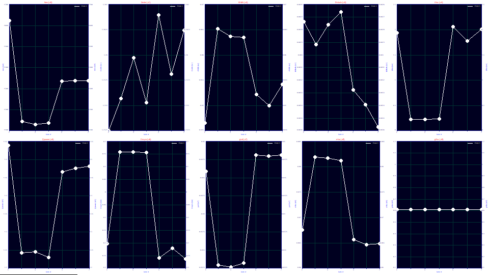
If you look at the third plot of a2, the Gaussian deconvolved widths, you see column 1 with the smallest width (and correspondingly highest theoretical plate count) in the Numeric Summary. The three column 3 replicates to the far right are next in width. The three column 2 replicates have the highest width (and thus the lowest theoretical plate count). There is a modest indication column 1 is in a better health than column 3.
If you look ay the fifth plot of a4, you see the width asymmetry. A width asymmetry of 2.0, means that the right side width will twice that of the left side. A width asymmetry of .25, means the right side width is only one-quarter of the left side. This is a massive difference in ZDD shape. It differentiates the poorly performing column 2 very strongly, but not the smaller differences between columns 1 and 3.
We would have expected the a5 power of decay term, that which impacts the fourth moment, to be the most important parameter fitted since it estimates the measure of overload. An a5 of 2, actually closer to 1.98 in practice, represents an overload-free analytic shape. An a5 of 1.0 represents a complete overload, that point where an envelope of overload (plateau between rise and fall) begins. For column 1, the a5 is 1.540. For column 3, the a5 ranges 1.467-1.481 across the three replicates. For the performance-diminished column 2, it is 1.231-1.246 across the replicates. This is what we expected this model to distinguish, the greater overload state in the column with poorer health.
The ZDD third moment adjustment, a6, is seriously impacted by the two separate left and right side widths. Here we see the poorly performing column with a vastly different a6, strongly positive instead of strongly negative.
With respect to the IRF, there are so many interactions in the higher moments that can impact the narrow width a7, we will look only at the wider a8 exponential width. It does not distinguish columns 1 and 3, but it does show column 2 with about a 1/4 higher exponential width. Something major in mass transfer, fluid dynamics, or adsorption-desorption is being impacted in column 2 and this is reflected in the exponential time constant of the IRF. In general, the higher width exponential term in an IRF tends to be remarkably stable. In analytic fitting, changing process variables such as temperature, additives, and analytic concentration moves the exponential width by at most a few percent. A full 25% increase in the exponential distortion does suggest massive differences in column function.
Overload State Deconvolutions
Click OK to close the Explore window. Select IRF Deconv. in the second Review window dropdown and Partial Deconv. in the third. Double click the first graph.
![]() Click the Hide Y plot in the graph's toolbar. Use the mouse to zoom in just the peak.
Click the Hide Y plot in the graph's toolbar. Use the mouse to zoom in just the peak.
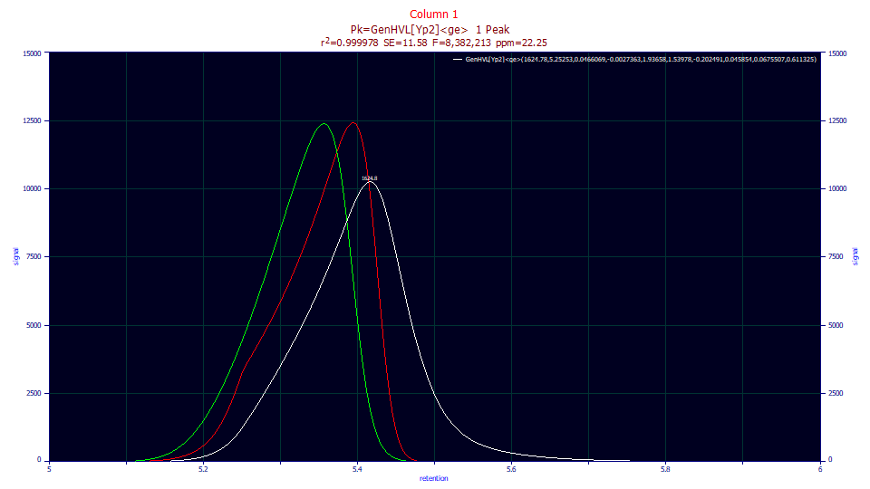
The white curve is the peak shape as eluted. The red curve is the peak with the IRF removed. You will note the unusual shape. This is due to the overload, to the ZDD's power of decay being less than two. When that fourth-moment influence is removed in the green curve, the pure HVL absent any form of overload, the shape is that of a fronted analytic peak. If you look the red peak closely, you see what appears to be a clean rise for about the first third when something very definitely happens to alter the shape.
Double click the graph to restore all plots. Double click the fourth graph. We will now see the deconvolution for the column in poor health.
![]() Click the Hide Y plot in the graph's toolbar. Use the mouse to zoom in just the peak.
Click the Hide Y plot in the graph's toolbar. Use the mouse to zoom in just the peak.
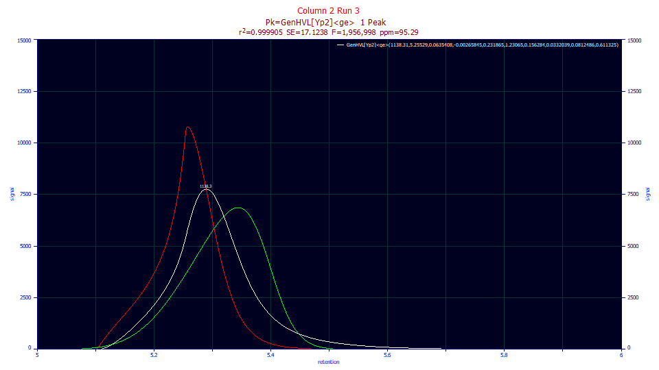
The white curve is again the peak shape as eluted. The red curve is the peak with the IRF removed. Remember that the <ge> convolution only adds the sum of a narrow and wider tailing. The red curve is that which remains after the tailing is removed from the white curve. If you further remove the fourth-moment factor of overload, restoring the power of two to the decay, and remove the ZDD third moment asymmetry, you are left with the green HVL. Note the center of the two green HVL peaks is close to identical, although the peak from the poorly performing column is wider. In this case, there is no portion of the rise of the red curve that looks normal before some form of interruption.
Deconvolution and Fitting
In these deconvolutions arising from fitting, the red curve can be viewed as an intermediate which reflects both an IRF absence and a ZDD presence. Different fits might produce a different red intermediate, depending on the specific IRF and ZDD assumed. In general, however, the white curve and the green curve are unlikely to change significantly. The green HVL is the pure chromatographic peak (for a Gaussian diffusion broadening).
Think of the fitting as a process in reverse. You first guess estimates of the green HVL. You then guess the non-idealities associated with the third and fourth moments of the ZDD upon which the Generalized HVL is based, and you get the red curve. You then guess the widths and area fraction of a narrow and wide instrument response function producing the added tailing. Those IRF parameter guesses will produce a final white curve that will initially be rather far removed from the eluted peak data. The guesses are then iteratively adjusted in n-dimensional parameter space until the white peak comes as close as possible to the original data.
Click OK to close the Review, OK to accept a saved GenHVL[Yp2]<ge> fit in the data file, and OK to acknowledge the revision in the file and OK once more to return to the main window.


 |