PeakLab v1 Documentation Contents AIST Software Home AIST Software Support
Fitting Hidden Peaks (Tutorial)
PeakLab offers the two methods for automatically finding hidden peaks in data. In the first of these, hidden peaks are found by the positive valued residuals between the placed peaks and data when equal areas are enforced. In the second, a smoothed second derivative data stream reveals hidden peaks at its minima. You can also, at your discretion, add and subtract peaks prior to fitting, and graphically or numerically adjust placements prior to fitting.
Importing the Data
![]() Click the Open button, the first button in the program's main toolbar. Select the file HiddenPeaksTutorial.pfd
from the program's installed default data directory (\PeakLab\Data).
Click the Open button, the first button in the program's main toolbar. Select the file HiddenPeaksTutorial.pfd
from the program's installed default data directory (\PeakLab\Data).
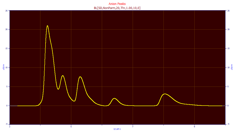
There are multiple levels of data in the data file:
Data to be Fitted (BL,DC) the data to be fitted, baseline corrected and IRF deconvolved
Data to be Fitted (BL) the data to be fitted, baseline corrected
Sectioned Data the sectioned area of data for the fitting (not as yet baseline corrected)
Reference Peak a sectioned reference peak, fronted and baseline-resolved, from early in the
elution - baseline corrected; for IRF estimation, this level contains a GenHVL<ge> fit with <ge>
IRF estimates
Transform X=X/1.87-1 dead-time computation for retention units
Imported Data the instrument data
We will be fitting only the two uppermost data levels, the Data to be Fitted (BL,DC) level with the IRF that was previously removed in the IRF Deconvolution procedure, and the adjacent Data to be Fitted (BL) level which contains the baseline-corrected data to be fitted, but where no IRF has been removed.
Since the uppermost (BL,DC) level has seen a Fourier deconvolution to remove the IRF, any hidden peaks should be at least slightly more apparent as a consequence of the sharpening arising from the deconvolution. This level will be quickly fitted to the closed form GenHVL and HVL models.
The adjacent (BL) level still contains the IRF distortions. Any hidden peaks will be at least somewhat
harder to see visually. The peaks will also have to be fitted to IRF convolution integral models. We will
use the GenHVL<ge> model.
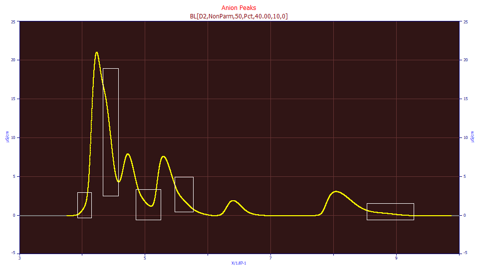
With some experience, hidden peaks are easily enough discerned visually. There is a chance there is a tiny peak hidden in the rise of the first local maxima peak. There is clearly a peak hidden in the decay of this first local maxima peak. The zone between the second and third local maxima peaks is suspect since there is a good separation but the peaks do not decay anywhere close to the baseline. The third local maxima peak has a tiny hidden peak in its decay, and the fifth local maxima peak has a very long sloping tail indicative of a tiny peak as well.
If you are curious, we did cherry-pick this data, but we did so with the intention of finding the most onerous and challenging example of hidden peaks we had available to us. Here we have five local maxima peaks and five quite ugly hidden peaks. We will note that two or more hidden peaks in sequence represent a kind of worst-case scenario, and those can be successfully fitted, but not with any form of automated detection, such as we highlight in this tutorial.
For this data, an instrument integration would process the five local maxima peaks, dropping intersecting tangents, and integrating those x-locations as the start and stop of each of the peaks. In our simple visual analysis, we have identified three hidden peaks which we can be reasonably certain exist, and two more which are perhaps likely but somewhat less certain. If our analysis is correct, only the fourth of the five local maxima peaks is likely to have a correct instrument integration.
For the purpose of this tutorial, let us say that it is as important to determine the number of components as well as their specific quantities.
Fitting the GenHVL to Hidden Peaks Using the Residuals Method
Change the Data Levels dropdown to Data to be Fitted (BL,DC). We will first fit the IRF deconvolved data. Since we can fit closed-form models, the fitting will be fast.
Click the Hidden Peaks - Residuals button in the Fit Peaks section of the dialog. You will now see the peak placement screen. Ensure the following settings are selected:
Baseline
No Baseline
Peak Detection
Savitzky-Golay
Set Sm n(1)
to 10
Peak Type
Select Chromatography
in the first dropdown
Select GenHVL as the model in the second dropdown
Scan
Set the Amp %
threshold to 1.5 % (local maxima peaks 1.5% of maximum amplitude
and higher are added)
Set the Res % threshold to 5
% (residual peaks 5% of maximum positive residuals and higher are added)
Check Add Residuals (we want the peaks from
the residuals added to the placement)
Check Use Baseline Segments (we will constrain
the fitting so that the a2
and a3
parameters are constant for each baseline resolved data segment)
Be sure Use IRF,ZDD is checked
Vary
Uncheck both width a2
and shape a3, all others should be unchecked as well
With the Use Baseline Segments fitting, peaks are grouped by baseline resolved segments and each will be fitted separately. When the a2 width and a3 chromatographic asymmetry are shared as is the case here, they are only shared on a per segment basis, and not across the full data set. You will see three baseline resolved segments with a blue, red, and green background. All peaks in the blue zone will have a common a2 and a3, the peak in the red zone will have its own a2 and a3, and the two peaks in the green will share their own a2 and a3. In this type of hidden peak fitting, we assume there is not enough information available to fit independent a2 and a3 widths for each peak. We will, however, attempt this a bit further along in thus tutorial.
Click the ZDD button. If you made modifications to the ZDD defaults prior to this tutorial for your own fitting, please use the Save button to save your ZDD values before resetting the defaults. Click the Defaults button. These are based on retention scale averages of modern IC data for each of the ZDDs built into the program. Check the Lock button to the right of the asym adjust for the GenHVL. We want to use the historical asymmetry (zero-distortion third moment non-ideality) for a4. Click OK.

The algorithm did find four of the five hidden peaks we visually identified and precisely where we felt they existed.
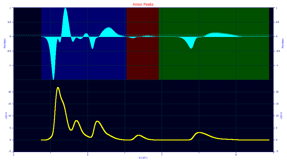
One look at the residuals plot reveals no hope of this method detecting the tiny peak hidden in the initial rise of the first peak. No level of residual threshold will make any difference, at least with this model and the default zero distortion density asymmetry which we locked at its historical default value. Note the four strongly defined positive value residuals shapes. The only other positive shape (suggesting an unaccounted peak) is very small, and is associated with the fourth local maxima peak.
Click the Peak Fit button in the lower left of the dialog to open the fit strategy dialog. Select the Fit with Reduced Data Prefit, Cycle Peaks, 2 Pass, Lock Shared Parameters on Pass 1. Be sure the Fit using Sequential Constraints box checked. Click OK.
If you are fitting any peak model bearing an IRF or ZDD parameter(s), you will almost always wish to use a 2-Pass option where the main peak parameters are first estimated while the starting estimates for the IRF and/or ZDD are held constant. For this kind of fitting, the Cycle Peaks option (where individual fits are performed of lower amplitude peaks) is probably essential.
For this hidden peak fitting, you will probably wish to check the Iteration Update button even though it somewhat slows the fitting. There is a graphical update of the fit with each iteration where an improvement occurs. This will allow you to see the different peaks falling into place within the fitting. Click Review Fit when the fitting is finished.
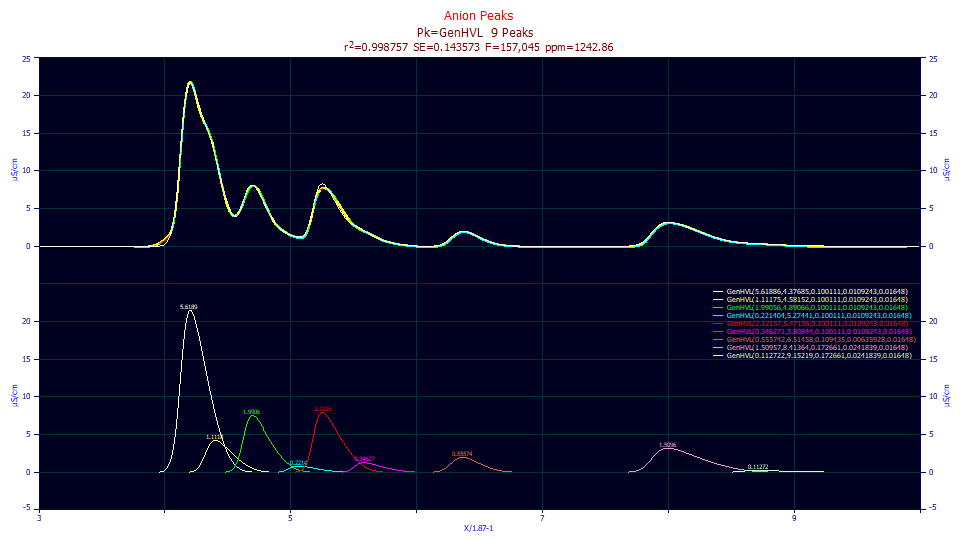
The 1242 ppm reflects the absence of the first hidden peak, which is indeed obvious in this fit, as well as the fact we forced all six peaks in the first (blue background) segment of the data to share a common a2 and a3. We know the a2 width generally increases with elution time. We also know that the a3 distortion generally has a continuous transition from negative (intrinsically fronted) to positive (intrinsically tailed) values; there is typically a retention where a3 crosses zero, and the the magnitude or absolute value of a3 increases to each side of this zero a3 point. We deliberately gave up a measure of fitting accuracy to enforce consistent results (to avoid overfitting the data).
Click the Numeric button if the Numeric Summary window is not currently displayed. Choose Select Only Fitted Parameters from the Options menu.
Fitted Parameters
r2 Coef Det DF Adj r2 Fit Std Err F-value ppm uVar
0.99875714 0.99875278 0.14344732 239,401 1242.86315
Peak Type a0 a1 a2 a3 a4
1 GenHVL 5.61885728 4.37685298 0.10011121 0.01092433 0.01648000
2 GenHVL 1.11175462 4.58152251 0.10011121 0.01092433 0.01648000
3 GenHVL 1.99056171 4.89065879 0.10011121 0.01092433 0.01648000
4 GenHVL 0.22140442 5.27440589 0.10011121 0.01092433 0.01648000
5 GenHVL 2.12156664 5.47155561 0.10011121 0.01092433 0.01648000
6 GenHVL 0.34627100 5.80843943 0.10011121 0.01092433 0.01648000
7 GenHVL 0.55574215 6.51457520 0.10943526 0.00635928 0.01648000
8 GenHVL 1.50957476 8.41363971 0.17266141 0.02418394 0.01648000
9 GenHVL 0.11272249 9.15219314 0.17266141 0.02418394 0.01648000
Note that the first six peaks share a common a2 width, the seventh peak has its own, and the last two peaks share a width. Overall the peaks are expected to increase in value, and we see such for the three segments. Note that the shared a3 value for the low amplitude fourth peak is grayed, meaning that it failed the 95% confidence significance test. This is not an issue when such a value is shared across multiple peaks and those with a stronger presence in the data fit to significance.
At this point we will note that this may be as far as you are able to go with this type of hidden peak fitting, depending on the S/N of the data. In this case, we can press further. We will add the missing peak, and further allow the a2 and a3 peak values to vary on a per peak rather than per segment basis, understanding the possibility that in doing so, the hidden peaks may adopt wild and inconsistent widths and shapes.
Click OK to close the Review, and if needed, check Save updated information to the current data file when adding fits. Click OK, accepting the default name for the fit. Click OK to confirm. You will now be back in the placement screen. The peak estimates have been updated to reflect the fitted values.
PeakLab offers graphical peak adjustment. A left click in the placement screen where the individual peaks are shown will place a new peak. There are also peak anchors which you can use to drag placed peaks to more appropriate locations, widths, and asymmetries.
Click a point just to the left of the first large peak (white), near where it first rises, at the location where we believe the missing peak should be located. A tenth peak has been added at the location where you clicked the mouse.
Place the mouse on the new anchor at the apex of this peak, left click and hold, sliding the peak up and down, left and right, to where you feel it will come closest to matching the data in the upper graph and then release. Repeat this a few times to get the placed peak and data as close to matching in the upper graph as possible.
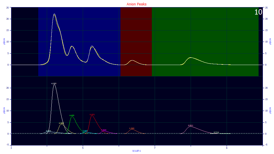
There will now be an initial sky-blue first peak in the sequence that should look similar to the plot above.
We could proceed now with the fit, but to ensure we each see exactly the same fit, we manually adjust the parameter values for this first peak. Right click this new peak anchor.
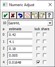
Enter the values as per the dialog above. Uncheck the share for a2 and a3. Click OK (green checkmark).
Right click the graph and select Set Common Parameters Across Peaks for this Data Set from the popup menu.
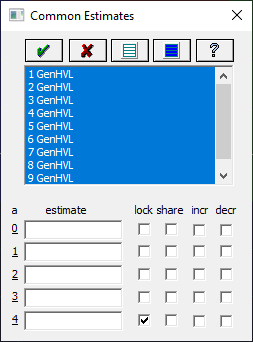
![]() Click the Select All Peaks button. Uncheck the share for the a2 width
and a3 chromatographic shape parameters. You will need to check the lock on a4
ZDD asymmetry parameter to ensure that no shared value is fitted.
Click the Select All Peaks button. Uncheck the share for the a2 width
and a3 chromatographic shape parameters. You will need to check the lock on a4
ZDD asymmetry parameter to ensure that no shared value is fitted.
![]() Click the OK button to accept the changes.
Click the OK button to accept the changes.
Click the Peak Fit button and then click OK to start the fitting. Click Review Fit when the fitting is finished.
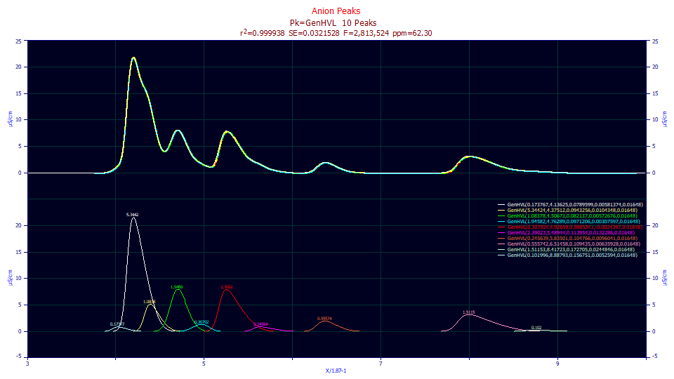
Click the Numeric button if the Numeric Summary window is not currently displayed. Choose Select Only Fitted Parameters from the Options menu.
Fitted Parameters
r2 Coef Det DF Adj r2 Fit Std Err F-value ppm uVar
0.99993770 0.99993734 0.03215276 2,813,524 62.2959295
Peak Type a0 a1 a2 a3 a4
1 GenHVL 0.17376728 4.13625461 0.07895990 0.00581374 0.01648000
2 GenHVL 5.34423783 4.37512413 0.09432556 0.01043480 0.01648000
3 GenHVL 1.08377960 4.50672804 0.08213699 0.00572676 0.01648000
4 GenHVL 1.94581515 4.76288602 0.09712060 0.00307597 0.01648000
5 GenHVL 0.30792424 4.92658771 0.08853408 -0.0024397 0.01648000
6 GenHVL 2.39023213 5.48943763 0.11395357 0.01322855 0.01648000
7 GenHVL 0.24563932 5.83500935 0.10476568 0.00960410 0.01648000
8 GenHVL 0.55574215 6.51457520 0.10943526 0.00635928 0.01648000
9 GenHVL 1.51152554 8.41722876 0.17270500 0.02448455 0.01648000
10 GenHVL 0.10199589 8.88793318 0.15675098 0.00525940 0.01648000
We now have a much better fit. The F-statistic has increased from 239K to 2.8 million. An F-statistic estimates the modeling efficacy, taking into account the number of parameters used to realize a given goodness of fit. Although this is an exceptional fit, it is hardly a perfect one. We still have one a3 value, on this added peak, which fails significance. The a3 parameter, now independent, varies for each peak. Note that the fifth peak (cyan) has a fronted a3 where all others are tailed.
Click OK to close the Review. Click OK, accepting the default name for the fit. Click OK to confirm. Click OK to return to the main window.
Fitting the GenHVL to Hidden Peaks Using the Second-Derivative Method
Click the Hidden Peaks - Second Derivative button in the Fit Peaks section of the dialog. Ensure the following settings are selected:
Baseline
No Baseline
Peak Detection
Savitzky-Golay
Set Sm n(1)
to 40
Peak Type
Select Chromatography
in the first dropdown
Select GenHVL as the model in the second dropdown
Scan
Set the Amp %
threshold to 1.5 % (local maxima peaks 1.5% of maximum amplitude
and higher are added)
Set the D2 % threshold to -5
% (-5% of maximum magnitude D2 well, normalized D2 = +.05)
Check Use Baseline Segments (we will constrain
the fitting so that the a2
and a3
parameters are constant for each baseline resolved data segment)
Be sure Use IRF,ZDD is checked
Vary
Uncheck both width a2
and shape a3, all others should be unchecked as well
The second derivative curve used for peak placement requires a higher smoothing, even when the data have a high S/N. We use an 81 point Savitzky-Golay window for the D2 curve. A peak exists where there are minima in a smooth second derivative curve. With smoothing, the minima may exist, but they may not decay below the D2=0 threshold. Normally, you would specify a value such as 2%. This sets a threshold at 2.0% of the highest magnitude minimum in the D2 curve shown in the lower graph. The D2 curve is normalized to -1. This means that a D2 well must be deeper than -.02 to be counted as a peak. Here we set a negative value, -5%, acknowledging that the D2 smoothing is such that the wells in the smoothed data never quite drop below 0.0. The -5.0 means that any D2 wells +.05 and below are treated as peaks. For this data set, at least +3% is needed to find all five of the hidden peaks.
We again use the Baseline Segments fitting where peaks are grouped by baseline resolved segments and fitted separately. Note that there will be a -1.0 normalized maximum D2 well in each of the segments.
Note also that the GenHVL a4 asymmetry is still locked at the IC default from the prior fits.
Here we fit all 10 peaks from the start. We begin with a2 and a3 shared on a per-segment basis as we did with the residuals method fits.
Click the Peak Fit button in the lower left of the dialog to open the fit strategy dialog. We will again use the Fit with Reduced Data Prefit, Cycle Peaks, 2 Pass, Lock Shared Parameters on Pass 1 strategy. Again, be sure the Fit using Sequential Constraints box checked. Click OK. Click Review Fit when the fitting is finished.
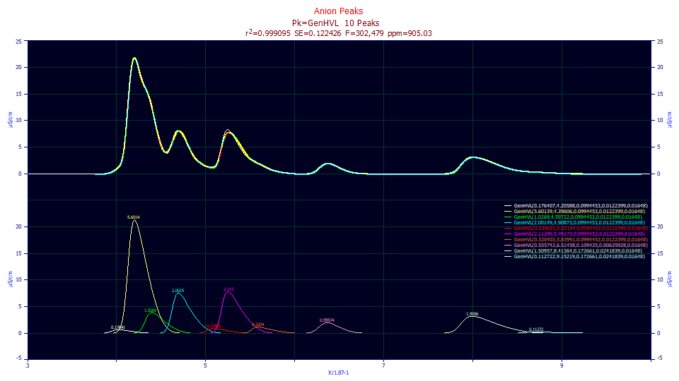
Unlike the residuals fit where a2 and a3 were shared on a per segment basis, we now have this tenth peak included and 905 ppm instead of 1246 ppm unaccounted variance.
Click the Numeric button if the Numeric Summary window is not currently displayed. Choose Select Only Fitted Parameters from the Options menu.
Fitted Parameters
r2 Coef Det DF Adj r2 Fit Std Err F-value ppm uVar
0.99909497 0.99909154 0.12242626 302,479 905.025498
Peak Type a0 a1 a2 a3 a4
1 GenHVL 0.17640722 4.20587831 0.09944530 0.01223992 0.01648000
2 GenHVL 5.60139414 4.39605673 0.09944530 0.01223992 0.01648000
3 GenHVL 1.02689968 4.59721633 0.09944530 0.01223992 0.01648000
4 GenHVL 2.00149074 4.90873379 0.09944530 0.01223992 0.01648000
5 GenHVL 0.23902141 5.32133922 0.09944530 0.01223992 0.01648000
6 GenHVL 2.11298828 5.49172817 0.09944530 0.01223992 0.01648000
7 GenHVL 0.32040291 5.83991133 0.09944530 0.01223992 0.01648000
8 GenHVL 0.55574215 6.51457520 0.10943526 0.00635928 0.01648000
9 GenHVL 1.50957476 8.41363971 0.17266141 0.02418394 0.01648000
10 GenHVL 0.11272249 9.15219314 0.17266141 0.02418394 0.01648000
As in the residuals fit, the peak between local maxima peaks 2 and 3, the one inferred only from the failure to drop to a baseline, has an a3 chromatographic asymmetry which fails significance. At this weak goodness of fit, the first peak, little more than a hint in the rise of the much larger first local maxima peak, fails significance for all parameters except its location.
Click OK to close the Review. Click OK, accepting the default name for the fit. Click OK to confirm.
We will again use the common parameters option to change the a2 and a3 parameters to where they vary on a peak by peak basis. Note that the placement now consists of much more accurate estimates from this first segmented fit. If you make any change in the left panel of the dialog a new rescan and placement will occur. Since we want to preserve the fitted estimates from this first fit for the next more intricate one, we must use this common parameters option.
Right click the placement graph and select Set Common Parameters Across Peaks for this Data Set from the popup menu.
![]() Once again, click the Select All Peaks button and uncheck the share for the a2 width
and a3 chromatographic shape parameters. Check lock on the a4 ZDD asymmetry
parameter to ensure that no shared value is fitted.
Once again, click the Select All Peaks button and uncheck the share for the a2 width
and a3 chromatographic shape parameters. Check lock on the a4 ZDD asymmetry
parameter to ensure that no shared value is fitted.
![]() Click the OK button to accept the changes.
Click the OK button to accept the changes.
Click the Peak Fit button and then click OK to start the fitting. Click Review Fit when the fitting is finished.
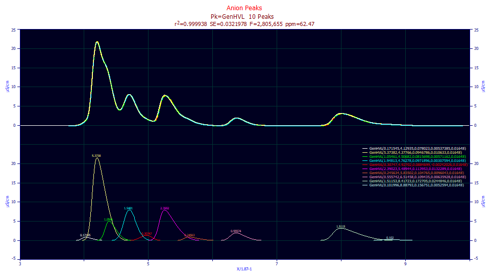
We have almost the same goodness of fit that we saw with the residuals fits where a2 and a3 were allowed to vary. The small differences can arise when a parameter fails significance, where it cannot be statistically assumed to be non-zero to a specific confidence.
Click the Numeric button if the Numeric Summary window is not currently displayed. Choose Select Only Fitted Parameters from the Options menu.
Fitted Parameters
r2 Coef Det DF Adj r2 Fit Std Err F-value ppm uVar
0.99993753 0.99993716 0.03219781 2,805,655 62.4706334
Peak Type a0 a1 a2 a3 a4
1 GenHVL 0.17154523 4.12935061 0.07802301 0.00537385 0.01648000
2 GenHVL 5.37381508 4.37766370 0.09467865 0.01063303 0.01648000
3 GenHVL 1.05461319 4.50681860 0.08156979 0.00571162 0.01648000
4 GenHVL 1.94813019 4.76277762 0.09718956 0.00307594 0.01648000
5 GenHVL 0.30747012 4.92702094 0.08846986 -0.0024203 0.01648000
6 GenHVL 2.39022572 5.48944379 0.11395265 0.01322890 0.01648000
7 GenHVL 0.24563394 5.83501538 0.10476481 0.00960430 0.01648000
8 GenHVL 0.55574215 6.51457520 0.10943526 0.00635928 0.01648000
9 GenHVL 1.51152554 8.41722876 0.17270500 0.02448455 0.01648000
10 GenHVL 0.10199589 8.88793315 0.15675098 0.00525940 0.01648000
This is a good point to put the a3 significance failures in context. A failed significance in a3 does not mean the peak cannot be confirmed. Its area, location and width are statistically significant, meaning non-zero within the default 95% confidence. It is the a3 shape that cannot be confirmed as non-zero, and a zero a3 is still a valid peak. It simply cannot be determined from the fit whether or not its intrinsic shape is fronted or tailed.
A true global minimum is usually realized for all fits of baseline resolved peaks and overlapping peaks with a reasonable local maxima. The innovations in the fitting algorithm were designed to ensure this. When peaks are strongly hidden, however, a number of local minima may exist, and since there are few data features to guide the hidden peak to this optimal solution, a local minima, a non-optimum result may be found in the fitting.
Peak Type a0-62.47ppm a0-62.29ppm a0-905ppm a0-1242ppm
1 GenHVL 0.17154523 0.17376728 0.17640722
2 GenHVL 5.37381508 5.34423783 5.60139414 5.61885728
3 GenHVL 1.05461319 1.08377960 1.02689968 1.1117546
4 GenHVL 1.94813019 1.94581515 2.00149074 1.9905617
5 GenHVL 0.30747012 0.30792424 0.23902141 0.22140442
6 GenHVL 2.39022572 2.39023213 2.11298828 2.12156664
7 GenHVL 0.24563394 0.24563932 0.32040291 0.34627100
8 GenHVL 0.55574215 0.55574215 0.55574215 0.55574215
9 GenHVL 1.51152554 1.51152554 1.50957476 1.50957476
10 GenHVL 0.10199589 0.10199589 0.11272249 0.11272249
If we compare the four different fits for area, we see differences but in general the agreement is good. The hidden peaks are underlined. Bear in mind that the conventional instrument integration would give you five components and no accuracy on four of those five components. Here we have a strong degree of confidence that we have ten peaks present, and we know the approximate amount of each of the components present.
Click OK to close the Review. Click OK, accepting the default name for the fit. Click OK to confirm. Click OK to return to the main window.
As you will have noted in this tutorial, two of the worst kinds of hidden peaks are those which are small and buried in the rise of much larger peaks, and those that fill the gap between two peaks whose only telltale is the lack of baseline. For those reasons, this data set really does represent an fair extreme with respect to hidden peaks.