PeakLab v1 Documentation Contents AIST Software Home AIST Software Support
Fitting Preparative (Overload) Peaks (Tutorial)
In this tutorial we will fit high-overload preparative shapes.
The Challenge of Fitting Overload Shapes
Of all the types of chromatographic peaks PeakLab can model, these peaks have proven to be the most challenging to fit to the near zero error we illustrate in the other types of tutorials. In an overload peak, the eluted shapes arise from the column and/or the detector function being saturated. In effect, the expected peaks are not seen because of a breakdown in either the column, the detector, or both. The high amount of eluting solute is processed very differently in this condition of saturation.
PeakLab's overload models are true theoretical chromatographic convolution models which address this saturation or breakdown and seek to reconstruct the peaks that would have been seen if the column and detector could fully manage the higher concentrations. The models perform the same deconvolutions as we observed with the constant mobile phase and gradient HPLC analytic peaks in the gradient peak tutorials.
In order to deconvolve an overload shape, we must fit a twice-generalized chromatographic model (one which addresses both third and fourth moments) just as we do for fitting the compressed shape of HPLC gradient peaks. In this instance, however, the fourth moment-related power of decay is employed in the opposite direction. Instead of fitting a higher power of fourth moment-related decay that represents the compression, we fit a lower power of fourth moment-related decay that represents a dilation. This dilation manages this overload state and produces the overload shapes seen in preparative chromatography.
Just as with fitting constant mobile phase analytic peaks, the IRF tailing must be addressed by fitting an IRF in a convolution integral. Unlike a gradient compression which cancels or offsets much of the IRF tailing, an overload state does the opposite, mathematically speaking, the dilation producing significantly increased tailing. Although we can modify the ZDD (zero distortion density) with this power of decay dilation to produce the overall core shape of the overload envelope, we cannot manage this inflated measure of tailing without fitting an <irf> convolution integral.
We also know that multiple non-idealities in fluid flow, mass transfer, and detection enter into the IRF components. We know that even the two component <ge>, <e2>, and <pe> IRFs we routinely use for analytic peaks represent simplifications that will not fully capture the error arising from these different distortions or non-idealities. If the tailing arising from the IRF is much increased, we would expect any error in fitting the IRF portion of the peak's tailing to likewise be higher.
The PeakLab overload models should be more than sufficient for you to characterize preparative peaks with high overload shapes, and to effectively estimate parameters that quantify overload and system performance.
Importing the Data
![]() Click the Open button, the first button in the program's main toolbar. Select the file OverloadTutorial.pfd
from the program's installed default data directory (\PeakLab\Data).
Click the Open button, the first button in the program's main toolbar. Select the file OverloadTutorial.pfd
from the program's installed default data directory (\PeakLab\Data).
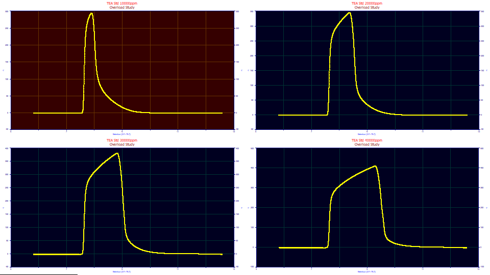
The data consist of four TEA overload peaks with concentrations varying between 1 and 4 % (10000, 20000, 30000, and 40000 ppm in the titles). The dead time transform and baseline correction have already been applied. The data are thus ready for fitting.
Click View and Compare Data. Check Single/Contour, check None for Normalization, and check Force Zmin=0.
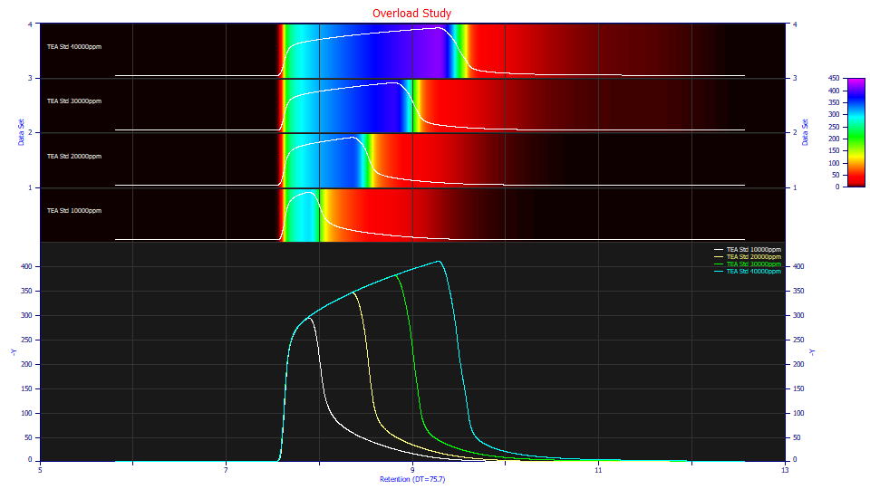
Both the contour and non-normalized data plots clearly confirm the overload state. The additional concentration goes into the overload envelope. Note the differences in the strong tailing. If you were to place a tangent line on the decay of each of the envelopes, you see the tailing beginning at about 140, 110, 95, and 70 Y signal values across the four samples. If we treat this tailing as an IRF, the exposed portion of the IRF is greatest on the lowest concentration sample, and smallest on the highest concentration sample. If you look at the contour, the tailing appears more drawn out for the higher concentration samples. The tailing is important because fitting the IRF is essential in accurately modeling overload peaks.
Click OK to exit the View and Compare Data option.
The GenHVL[Yp] Overload Models
The twice generalized Gen2HVL (fitting both third moment and fourth moment effects) effectively manages these overload shapes. The Gen2HVL model's ZDD (zero distortion density) defines the a1 location parameter as the mean of the generalized error ZDD. The [Y] ZDD retains the a1 as the mean of the underlying Gaussian and we have chosen to use this form of the [Y] ZDD for the overload models.
When the power of decay (the fourth moment a4 term) in the [Y] generalized error class of ZDD drops from 2.0 toward 1.0, this dilation produces a progression similar to those in the sequence above. In fact, by the time an 'envelope' has fully formed, this fourth moment decay parameter fits to very close to 1.0, a ZDD which is a double-sided exponential or Laplace density.
In order to fit overload shapes, we require special versions of the [Y] ZDD general chromatographic models:
The GenHVL[Yp] (the appended 'p' for 'preparative') is identical to the GenHVL[Y] but offers a different starting estimate algorithm which assumes a high overload shape. In order to ensure the convergence of the non-linear fitting to an optimal solution, the starting estimates must be specific for this condition of overload.
The GenHVL[YpE] model is a simplification of the GenHVL[Yp] which assumes this generalized Laplace or double-sided exponential ZDD. It should only be used if a full overload envelope is present.
The GenHVL[Yp2] model is a modification of the GenHVL[Yp] where there are two widths fitted, a width for the peak consisting of the rise to the apex, and a separate width for the peak which decays from the apex. Although an additional parameter is required, this model can often be fitted successfully, and with much better goodness of fits. Like the GenHVL[Yp] model, the GenHVL[Yp2] can be used for partial overload envelopes.
The GenHVL[Yp2E] model is a simplification of the GenHVL[Yp2] which like the GenHVL[YpE] assumes this generalized double-sided exponential for the ZDD. It should also only be used if a full overload envelope is present.
As we now fit these overload shapes, please note that all of these overload models are generalized chromatographic models which use the common chromatographic distortion mathematics, just as was true of the models used in all of the other tutorials. In fact, with the proper starting estimates, this [Y] generalized error class of ZDD, can successfully fit virtually any chromatographic shape: analytic GC and LC peaks, gradient HPLC peaks, and overload preparative peaks. This two-higher moment class of chromatographic model could easily be deemed a universal model were it not for the fact the analytic peaks generally require only a third moment adjustment. This is why the GenHVL or GenHVL[Z] (the [Z] ZDD the basic variant with a1 as the mean of the underlying Gaussian), simplifications of the [Y] models, are used for analytic peaks. No fourth moment adjustment is needed.
For overload shapes, we require a ZDD zero distortion density with exceptionally 'fat' tails, a high fourth moment.
Fitting the GenHVL[Yp]<e2> Model
We must fit an IRF convolution integral to address the extensive tailing present in these overload peaks. Here we will use the <e2> IRF, the two component sum of first order exponentials. We thus begin by fitting the GenHVL[Yp]<e2> model, the twice-generalized overload model with the 'Yp' ZDD and the 'e2' IRF.
Click the Local Maxima Peaks button. You will use the other two peak fitting options only if you need help in finding hidden peaks. In data sets where the peaks are clearly defined by local maxima, each with a distinct apex, the simpler local maxima fitting should be used.
You will now see the peak placement screen. Ensure the following settings are selected:
Peak Detection
Set Sm
n(1) to 25
Peak Type
Select Chromatography
in the first dropdown
Select GenHVL[Yp]<e2> as the model in
the second dropdown
Scan
Set the Amp %
threshold to 1.5 %
Leave Use Baseline Segments unchecked
Be sure Use IRF,ZDD is checked
Vary
Leave width a2
and shape a3 checked, all other unchecked
You will note that each of the data sets has an automatic placement whose estimated parameters assume a strong overload shape.
Click the IRF button. If you made modifications to the IRF defaults prior to this tutorial for your own fitting, please use the Save button to save your IRF values before resetting the defaults. Click the Defaults button. These are based on retention scale averages of modern IC data for each of the IRFs built into the program. Change the first <e2> starting estimate, e width-1 (tau), to 0.5. This is to accommodate the overload data's much greater width primary exponential. Click OK. The tailing is now somewhat better mapped.
Click the Peak Fit button in the lower left of the dialog to open the fit strategy dialog. Select the Fit with Reduced Data Prefit, 2 Pass, Lock Shared Parameters on Pass 1. Be sure the Fit using Sequential Constraints box checked. Click OK. If you are fitting any peak model bearing an IRF or ZDD parameter(s), you will almost always wish to use a 2-pass option where the main peak parameters are first estimated while the starting estimates for the IRF and/or ZDD are held constant. For this strategy to work well, these ZDD and IRF estimates will need to be somewhat close to the fitted values.
Uncheck the Iteration Update button to speed up fitting. This stops the graphical update with each iteration where an improvement in fit occurred.
The fits should only require a few seconds. Click Review Fit when the fitting is finished.
Reviewing the GenHVL[Yp]<ge> Model
The lower graph, by default, shows only the fitted curve, the As Fitted selection in the first dropdown. There are additional dropdowns where you can see different aspects of the fitted peak. Select the IRF Deconv. option in the second dropdown. This plots, in the first aux component color (red by default for most color schemes), the fitted peak with the IRF removed, the GenHVL[Yp], the peak you would see if there existed no system/instrumental distortion. The IRF attenuates the peak and dramatically changes the shape.
![]() Click the Hide Y2 plot in the graph's toolbar.
Click the Hide Y2 plot in the graph's toolbar.
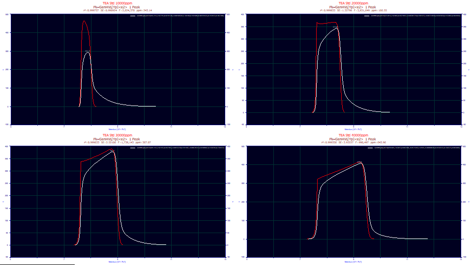
The two-component IRF, the area-weighted sum of first order exponentials, converts the unusual red shape, the GenHVL[Yp], to the white peaks registered by the instrument.
Change the third dropdown to Partial Deconv. The second auxiliary component color is usually green by default. For this model, the green peak (the partial deconvolution) is the pure HVL, the theoretical peak after the ZDD's third and fourth moment non-idealities are mathematically removed.
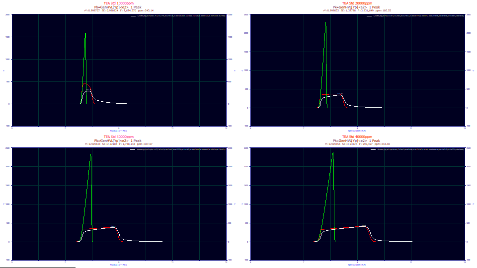
Please look closely the HVL deconvolution. This is the pure chromatographic peak you would expect to see if the the column/detector were immune to overload. As you will note, the green deconvolved HVL is sharply fronted. Even peaks with very little a3 chromatographic distortion at analytical concentrations will have that measure of fronting or tailing amplified by concentration. Deconvolved preparatory peaks should be strongly fronted, or strongly tailed, depending on the sign of a3.
Click Numeric to open the Numeric Summary and from the Options menu, choose Select Only Fitted Parameters and also check Deconvolved Moments and Advanced Area Analysis.
"TEA�Std�10000ppm"
Fitted�Parameters
r2�Coef�Det�� DF�Adj�r2���� Fit�Std�Err�� F-value������ ppm�uVar
0.99975686��� 0.99975643��� 0.99092398��� 2,624,370���� 243.142042
�Peak Type���������� ������a0���� ������a1���� ������a2���� ������a3���� ������a4���� ������a5���� ������a6���� ������a7���� ������a8��
����1�� GenHVL[Yp]<e2>�� 165.712367�� 7.62790616�� 0.02915358�� -0.0016850�� 1.56108587�� 0.16168679�� 0.49264681�� 0.00991622��0.53729199��
Deconvolved�Moments
�Peak�� Type�������� ���Area����� ���Mean����� ��StdDev���� �Skewness��� �Kurtosis��� �Amplitude�� ���Center�����
����1�� HVL��������� 165.712367�� 7.71770294�� 0.04489006�� -0.7019512�� 2.91901600�� 1649.72479�� 7.75823777��
Advanced�Area�Analysis
�Peak�� Type������������ ����Area���� ��%�Area���� �ApexAsym��� �NonOverlap1 ��%�PkArea�� �NonOverlap2 ��%�PkArea��
����1�� GenHVL[Yp]<e2>�� 165.706546�� 100.000000�� 1.47867118�� 88.3333028�� 53.3070690�� 58.3726815�� 35.2265393��
"TEA�Std�20000ppm"
Fitted�Parameters
r2�Coef�Det�� DF�Adj�r2���� Fit�Std�Err�� F-value������ ppm�uVar
0.99983345��� 0.99983316��� 1.32798346��� 3,831,649���� 166.545420
�Peak Type���������� ������a0���� ������a1���� ������a2���� ������a3���� ������a4���� ������a5���� ������a6���� ������a7���� ������a8��
����1�� GenHVL[Yp]<e2>�� 323.814430�� 7.62002945�� 0.03298375�� -0.0038178�� 0.98442511�� -0.0025486�� 0.45386384�� 0.03646563��0.33514355��
Deconvolved�Moments
�Peak�� Type�������� ���Area����� ���Mean����� ��StdDev���� �Skewness��� �Kurtosis��� �Amplitude�� ���Center�����
����1�� HVL��������� 323.814430�� 7.76191624�� 0.06365485�� -0.6934033�� 2.79079270�� 2333.81036�� 7.82965650��
Advanced�Area�Analysis
�Peak�� Type������������ ����Area���� ��%�Area���� �ApexAsym��� �NonOverlap1 ��%�PkArea�� �NonOverlap2 ��%�PkArea��
����1�� GenHVL[Yp]<e2>�� 323.807068�� 100.000000�� 0.46231684�� 229.137593�� 70.7636168�� 54.5986678�� 16.8614812��
"TEA�Std�30000ppm"
Fitted�Parameters
r2�Coef�Det�� DF�Adj�r2���� Fit�Std�Err�� F-value������ ppm�uVar
0.99963293��� 0.99963229��� 2.52106273��� 1,738,143���� 367.067242
�Peak Type���������� ������a0���� ������a1���� ������a2���� ������a3���� ������a4���� ������a5���� ������a6���� ������a7���� ������a8��
����1�� GenHVL[Yp]<e2>�� 501.196639�� 7.62492405�� 0.04796292�� -0.0093378�� 0.99198708�� -0.0067834�� 0.45070353�� 0.04086680��0.24302761��
Deconvolved�Moments
�Peak�� Type�������� ���Area����� ���Mean����� ��StdDev���� �Skewness��� �Kurtosis��� �Amplitude�� ���Center�����
����1�� HVL��������� 501.196639�� 7.85002070�� 0.09845306�� -0.6871550�� 2.75980363�� 2346.76645�� 7.95814291��
Advanced�Area�Analysis
�Peak�� Type������������ ����Area���� ��%�Area���� �ApexAsym��� �NonOverlap1 ��%�PkArea�� �NonOverlap2 ��%�PkArea��
����1�� GenHVL[Yp]<e2>�� 501.184448�� 100.000000�� 0.29514841�� 362.272018�� 72.2831722�� 50.2737025�� 10.0309782��
"TEA�Std�40000ppm"
Fitted�Parameters
r2�Coef�Det�� DF�Adj�r2���� Fit�Std�Err�� F-value������ ppm�uVar
0.99935605��� 0.99935491��� 3.93225491��� 990,502������ 643.954884
�Peak Type���������� ������a0���� ������a1���� ������a2���� ������a3���� ������a4���� ������a5���� ������a6���� ������a7���� ������a8��
����1�� GenHVL[Yp]<e2>�� 698.602806�� 7.63006608�� 0.06314201�� -0.0179053�� 1.01030860�� -0.0080049�� 0.45060925�� 0.04512322�0.19485141��
Deconvolved�Moments
�Peak�� Type�������� ���Area����� ���Mean����� ��StdDev���� �Skewness��� �Kurtosis��� �Amplitude�� ���Center�����
����1�� HVL��������� 698.602806�� 7.94467842�� 0.13539268�� -0.6823806�� 2.73911603�� 2385.63939�� 8.09634866��
Advanced�Area�Analysis
�Peak�� Type������������ ����Area���� ��%�Area���� �ApexAsym��� �NonOverlap1 ��%�PkArea�� �NonOverlap2 ��%�PkArea��
����1�� GenHVL[Yp]<e2>�� 698.568754�� 100.000000�� 0.22800778�� 509.408942�� 72.9218046�� 48.8806517�� 6.99725709��
We'll point out the key numeric items, and then explore the different relationships graphically.
Goodness of Fit
The fits vary from 166 ppm to 643 ppm unaccounted variance. This was realized with the twice-generalized [Yp] ZDD. We will seek to improve upon the error in a further revision of the [Yp] density in the second half of this tutorial. At this point, we note that the values are higher than we would prefer, and despite the IRF decreasing with overload (confirmed with a8, the area fraction of the IRF's very large width component), the error of fit increases.
a4 Dilation
The dilation is in parameter a4, the power of decay. It fit to 1.56 for the partial overload shape, and very close to 1.0 for all three of the full envelope (a plateau between the rise and decay) data sets. A 2.0 power of decay is that of the Gaussian, 1.0 that of an exponential. Note that a4 maps a constant dilation of 1.0 once a full envelope has formed, and varies between 2 and 1 as the overload increases. The a4 dilation maps the overload shape, but only until a full envelope has formed.
![v5_GenHVL[Yp]Dilation.png](v5_GenHVL[Yp]Dilation.png)
The View Function(X) option was used to insert the parameters from the second data set's fit, and vary the a4 parameter from 2.0, the blue peak with no overload truncation, to 1.0, the full overload dilation of this data set. If your preparative peak is one of a partial overload, the a4 parameter will likely give you the greatest measure of information with respect to overload.
a5 Statistical Asymmetry
Although it would appear that a5 also fits to nearly 0 for the full envelope fits, the statistical asymmetry in a ZDD, that which adjusts the third moment, is seldom insignificant.
![v5_GenHVL[Yp]Asymmetry.png](v5_GenHVL[Yp]Asymmetry.png)
We again used the View Function(X) option with the values from the last of the four fits (blue). The a5 asymmetry is -.008. We added four curves, -.004 (red), -.006 (amber), -.010 (green), and -.012 (violet). In the three full-envelope fits, a5 appears to track the amount of plateau. With respect to the strongly positive a5 in the first fit, we can only note the shape is still a long way from a plateau occurring.
a6-a8 <e2> IRF Parameters
The a7 high width exponential fits to a constant .45 in the three full envelope overload data sets. This is about ten times the width observed for this instrument with analytic peaks. Since it was apparent just from visual inspection that the amount of this IRF tailing was itself saturated (decreasing proportional to peak area), the a8 area fraction of this largest width component also measures the overload, albeit in a very different way. Unlike analytic peaks where the IRF is somewhat constant, it is far from such in overload shapes. With respect to a7, the smaller of the two exponential widths, we must refer to the analytic <e2> IRF of [tau 1=.007, tau 2=.044, areafrac1=.62]. The a7 parameter certainly fit to the higher analytic width in the three full envelope fits. In case you were wondering if the two exponentials are needed, you should fit the GenHVL[Yp]<e> model. The fits will be terrible: 2376 ppm to 13140 ppm. As we have shared throughout the tutorials, fitting the IRF is essential in high accuracy chromatographic modeling, and overload shapes have massive IRFs.
Click Explore. Since the data sets linearly increase with concentration, we can assess the trends by concentration using Data # for the x variable. We will look at a0-a3, the pure HVL deconvolved values in these plots.
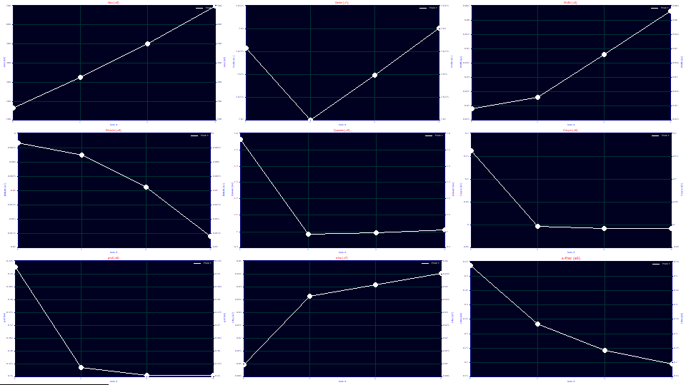
In the first graph, the a0 areas track concentration almost linearly.
One of the suggestions this model is theoretically sound for overload peaks is that the a1 locations are almost perfectly identical for the four vastly different overload shapes (the second graph scales a1 from 7.62 to 7.63).
The a2 widths increase with overload, and linearly once a full envelope is present. For this model, a2 is the SD width of the underlying Gaussian. For this data, you can right click any of the graphs of the fits and select AIA Import File Information for this Data Set. If you do so, you will see the original instrument's integration reporting widths that vary from 41 to 155 (the x units were in seconds), close to a factor of four. In the above plots, The a2 deconvolved Gaussian widths vary from .03 to .06, a factor of two. We will subsequently address in this tutorial this broadening of a2 with concentration.
The a3 chromatographic shape, strongly fronted, becomes more negative (more fronted) with concentration, another suggestion the model is tracking the overload well. Unlike the linearity of a3 with concentration observed with analytic peaks, the distortion increases with a power greater than 1. If a 0,0 point is inserted into the data (0 chromatographic distortion at 0 concentration), the data in this plot fit to a power of 2.15. In a full accuracy analytic fit, it is our experience that a3 is linear with concentration. Since these fits still have a measure of error, however, we cannot automatically assume overload produces a disproportionate measure of chromatographic distortion.
Click OK to close the Explore option.
![]() Click the Hide Y plot. You will now see only the fitted data.
Click the Hide Y plot. You will now see only the fitted data.
Using the mouse, zoom in the portion of the shape where the rise just begins. You can use any one of the shapes.
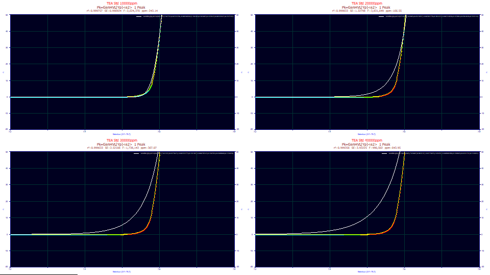
For the second through fourth data sets, there is a significant error in the initial rise. It increases with concentration, and corresponds with the poorer goodness of fit.
One solution is a third generalization of sorts, one which breaks the [Yp] zero distortion density into two separate components seamed at the apex. With a separate width for a each half of the density we can produce a much sharper rise. The GenHVL[Yp2] is an extension of the GenHVL[Yp] model which fits a separate width for the left and right sides of the peak.
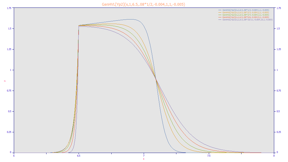
Here GenHVL[Yp2] width values have been adjusted to produce comparable shapes. The adjustable rise allows the lack of fit with the GenHVL[Yp] model to be corrected. Once a full envelope has formed, there is every reason to believe separate widths would be present in the ZDD.
Click OK to close the Review, and check Save updated information to the current data file when adding fits and click OK, accepting the default name for the fit. Click OK to confirm. You will now be back in the placement screen.
Fitting the GenHVL[Yp2]<e2>
We will now fit the GenHVL[Yp2] peak where the rise of the peak is independently fitted. The addition of an additional rise width parameter (expressed as a width asymmetry, a right-side width divided by a left-side width) changes the basic model from a six-parameter to a seven-parameter one. With a three parameter <e2> IRF added, we will be fitting ten total parameters instead of nine.
Click the Local Maxima Peaks button. Change the model to the GenHVL[Yp2]<e2>. Click the Peak Fit button in the lower left of the dialog to open the fit strategy dialog. Using the same settings as prior, click OK. The fits should only require a few seconds. Click Review Fit when the fitting is finished.
With As Fitted in the first dropdown, if it is not already present, place IRF Deconv. in the second dropdown Partial Deconv. in the third dropdown.
![]() Click the Hide Y2 plot in the graph's toolbar.
Click the Hide Y2 plot in the graph's toolbar.
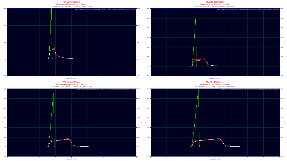
We now better model the nuances in the rise of the overload shape. In the GenHVL[Yp]<e2> fits, we had an average F-statistic of 2.3 million and 355 ppm unaccounted variance across the four fits. In these GenHVL[Yp2]<e2> fits, this one additional parameter resulted in an average F-statistic of 4.3 million and 147.1 ppm unaccounted variance. This one parameter dramatically increased the power and efficacy of the fitting.
We see the about the same red IRF-removed overload shapes, and similar green deconvolved HVL peaks which now increase in amplitude as well as in width with concentration. Intuitively, we would expect at least some increase in amplitude of the deconvolved HVL with the increasing concentration. With the better fitting of the narrow rise of the overload shape, the ZDD is changed in shape, and this is translating differently in the common chromatographic distortion mathematics.
Analyzing the GenHVL[Yp2]<e2>
Click Numeric to open the Numeric Summary and from the Options menu, choose Select Only Fitted Parameters and also check Deconvolved Moments and Advanced Area Analysis.
TEA�Std�10000ppm"
Fitted�Parameters
r2�Coef�Det�� DF�Adj�r2���� Fit�Std�Err�� F-value������ ppm�uVar
0.99975802��� 0.99975754��� 0.98866004��� 2,343,472���� 241.984910
�Peak Type������������� ������a0���� ������a1���� ������a2���� ������a3���� ������a4���� ������a5���� ������a6���� ������a7�����������a8�������a9����
����1�� GenHVL[Yp2]<e2>�� 165.699591�� 7.63050683�� 0.02978956�� -0.0017667�� 0.95382969�� 1.59973390�� 0.17562770�� 0.49175606��0.00753349��0.53574798��
Deconvolved�Moments
�Peak�� Type��������� ���Area����� ���Mean����� ��StdDev���� �Skewness��� �Kurtosis��� �Amplitude�� ���Center�����
����1�� HVL���������� 165.699591�� 7.72274368�� 0.04594607�� -0.7020460�� 2.91801540�� 1612.09703�� 7.76429890��
Advanced�Area�Analysis
�Peak�� Type������������� ����Area���� ��%�Area���� �ApexAsym��� �NonOverlap1 ��%�PkArea�� �NonOverlap2 ��%�PkArea��
����1�� GenHVL[Yp2]<e2>�� 165.693877�� 100.000000�� 1.48240727�� 86.6831801�� 52.3152586�� 57.8075050�� 34.8881360��
"TEA�Std�20000ppm"
Fitted�Parameters
r2�Coef�Det�� DF�Adj�r2���� Fit�Std�Err�� F-value������ ppm�uVar
0.99986153��� 0.99986126��� 1.21101447��� 4,095,737���� 138.471680
�Peak Type������������� ������a0���� ������a1���� ������a2���� ������a3���� ������a4���� ������a5���� ������a6���� ������a7�����������a8�������a9����
����1�� GenHVL[Yp2]<e2>�� 323.663348�� 7.61759861�� 0.03119390�� -0.0032068�� 1.36941334�� 0.99724048�� -0.0023158�� 0.46311223��0.03531645��0.32664782��
Deconvolved�Moments
�Peak�� Type��������� ���Area����� ���Mean����� ��StdDev���� �Skewness��� �Kurtosis��� �Amplitude�� ���Center�����
����1�� HVL���������� 323.663348�� 7.74673995�� 0.05864179�� -0.6957895�� 2.80457939�� 2526.30873�� 7.80823084��
Advanced�Area�Analysis
�Peak�� Type������������� ����Area���� ��%�Area���� �ApexAsym��� �NonOverlap1 ��%�PkArea�� �NonOverlap2 ��%�PkArea��
����1�� GenHVL[Yp2]<e2>�� 323.654534�� 100.000000�� 0.47529531�� 237.337848�� 73.3306111�� 53.8176966�� 16.6281300��
"TEA�Std�30000ppm"
Fitted�Parameters
r2�Coef�Det�� DF�Adj�r2���� Fit�Std�Err�� F-value������ ppm�uVar
0.99988660��� 0.99988637��� 1.40142174��� 5,001,186���� 113.404675
�Peak Type������������� ������a0���� ������a1���� ������a2���� ������a3���� ������a4���� ������a5���� ������a6���� ������a7�����������a8�������a9����
����1�� GenHVL[Yp2]<e2>�� 500.746011�� 7.61641433�� 0.04293464�� -0.0062967�� 2.47162746�� 1.02681407�� -0.0073440�� 0.51548379��0.03705191��0.20461323��
Deconvolved�Moments
�Peak�� Type��������� ���Area����� ���Mean����� ��StdDev���� �Skewness��� �Kurtosis��� �Amplitude�� ���Center�����
����1�� HVL���������� 500.746011�� 7.79795859�� 0.08191696�� -0.6944676�� 2.79675726�� 2801.67097�� 7.88458338��
Advanced�Area�Analysis
�Peak�� Type������������� ����Area���� ��%�Area���� �ApexAsym��� �NonOverlap1 ��%�PkArea�� �NonOverlap2 ��%�PkArea��
����1�� GenHVL[Yp2]<e2>�� 500.709732�� 100.000000�� 0.32286923�� 391.254383�� 78.1399597�� 47.1495800�� 9.41654954��
"TEA�Std�40000ppm"
Fitted�Parameters
r2�Coef�Det�� DF�Adj�r2���� Fit�Std�Err�� F-value������ ppm�uVar
0.99990538��� 0.99990519��� 1.50749340��� 5,993,965���� 94.6232557
�Peak Type������������� ������a0���� ������a1���� ������a2���� ������a3���� ������a4���� ������a5���� ������a6���� ������a7�����������a8�������a9����
����1�� GenHVL[Yp2]<e2>�� 697.884878�� 7.61608517�� 0.05551610�� -0.0110583�� 3.66288634�� 1.06518094�� -0.0085090�� 0.61958737��0.03773216��0.12932068��
Deconvolved�Moments
�Peak�� Type��������� ���Area����� ���Mean����� ��StdDev���� �Skewness��� �Kurtosis��� �Amplitude�� ���Center�����
����1�� HVL���������� 697.884878�� 7.85788217�� 0.10811585�� -0.6925349�� 2.78610988�� 2963.63704�� 7.97350246��
Advanced�Area�Analysis
�Peak�� Type������������� ����Area���� ��%�Area���� �ApexAsym��� �NonOverlap1 ��%�PkArea�� �NonOverlap2 ��%�PkArea��
����1�� GenHVL[Yp2]<e2>�� 697.677056�� 100.000000�� 0.26052019�� 559.392444�� 80.1792806�� 42.6207683�� 6.10895369��
Goodness of Fit
The most significant item is that the goodness of fit improves as the concentration and envelope increase, and as the high width IRF component diminishes. This is very encouraging since we investigated a large number of potential overload models, and with the exception of this GenHVL[Yp2] model, the goodness of fit worsened with the amount of overload, as the width of the envelope increased (as was observed with the GenHVL[Yp] fits at the start of this tutorial). The GenHVL[Yp2] did not substantially improve the fit of this first data set with its partial overload envelope. Note that an a4 width asymmetry of 1.0 is an equal width to the left and right of the apex, reducing to the GenHVL[Yp] model. On this first data set, a4 fit to 0.953 on this first peak, close to equal widths.
Click Explore.
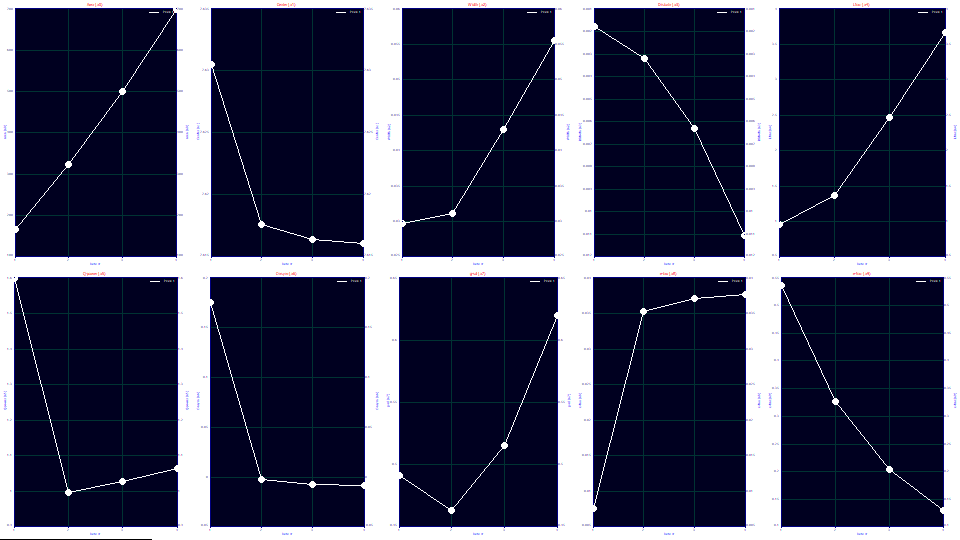
a1 Deconvolved Gaussian Center
The a1 deconvolved Gaussian mean is close to a constant for all four overload shapes, as was observed with the GenHVL[Yp] fits.
a2 Deconvolved Gaussian SD
The a2 deconvolved Gaussian SD increases with concentration and overload, again as was observed with the GenHVL[Yp] fits. If we look at the second moment of the deconvolved HVL (as an SD), we see a similar broadening with concentration and overload. The single width GenHVL[Yp] and two-width GenHVL[Yp2] models differ little in a2 values until the overload becomes extreme.
a3 Chromatographic Distortion
The a3 common chromatographic distortion increases with concentration (often linearly at analytic concentration). If we look at the third moment of the HVL peaks, all four shapes fit to a very narrow range around an extreme skewness of -.695. The a3 is far more sensitive for characterizing the strength of the fronting. With this GenHVL[Yp2] model, we also see the nonlinearity between a3 and concentration. The data fit to a power of 1.7 as compared to 2.15, not the linearity we perhaps wished to see, but an improvement.
a4 Width Asymmetry
The new parameter a4 is a width-based asymmetry, the right side width divided by the left side width. This parameter also strongly tracks the overload, linearly with a full envelope. For the last of the data sets, the a4=3.66 width asymmetry means that the right side of the peak is computed using a width of a2*a4/(1+a4) or .0436 and the left side of peak is computed using a width of a2/(1+a4) or .0119. The right side width of the [Yp2] ZDD density is 3.66x larger than the left side.
a5 Power of Decay
The a5 remains close to 1.0 for the full overload envelope data sets, and at 1.60, we see close to the GenHVL[Yp] 1.56 power of decay value for the first data set with the partial envelope. In both the GenHVL[Yp] and GenHVL[Yp2] fits, the power of decay increased slightly with concentration for the full envelope fits. With the separate rise and decay widths, this deviation from 1.0 is greater with the GenHVL[Yp2] model.
a6 Statistical Asymmetry
The first partial overload data set fits to a strong right-skewed asymmetry. The three full overload sets fit to slightly negative values as did the GenHVL[Yp] fits.
a7, a8, a9 <e2> IRF
Both of the effects we saw in the visualize step are confirmed. Unlike the GenHVL[Yp] fits, the two width fits produce the more extended a8 widths we saw in the original contours of the tails in the data. This a8 exponential component which produces the huge tailing now increases with concentration. The amount of the component a9 diminishes with concentration as did the single-width fits.
Change the y variable to Moments DC2. We will see plots of zeroth through fourth moments for the green deconvolved HVL peaks, the peaks above that represent the true peaks if the column/detector had an infinite capacity (no overload state).
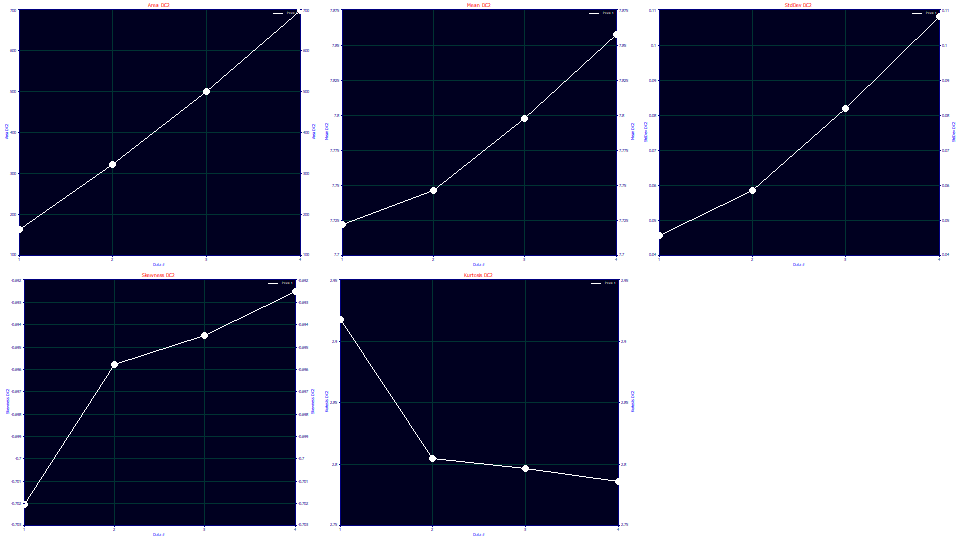
The pure HVL mean and standard deviations increase with overload, but linearly only for three samples with the full overload envelope shape (the power of decay or dilation near 1.0).
The HVL skewness reflects the very strong fronting and is nearly constant, -.70 to -.69. Even these tiny differences track close to linearly. The kurtosis of the HVL peaks drops from 2.92 to 2.79 across the four samples. HVL chromatographic peaks normally decay near the kurtosis of a Gaussian or higher, but strongly fronted chromatographic peaks are exceptions with thinner tails. Here, the higher the concentration, the more the kurtosis drops below the 3.0 of the Gaussian.
HVL Deconvolved Moments
These are also reported in the Deconvolved Moments section of the Numeric Summary. The green HVL peaks recovered by the deconvolution within the fitting have a narrower mean 7.72-7.85 as compared to the 7.71-7.94 range on the GenHVL[Yp] model. The skewness is very close to constant across all of the peaks. The kurtosis is thinner than Gaussian and thins further with the increased fronting, but only slightly once a full envelope is formed.
If we look at the GenHVL[Yp2] amplitude succession 1612-2526-2801-2963, as compared to the GenHVL[Yp]'s 1649-2333-2346-2386 ,we see an improved sharpened deconvolution closer to expectation.
Advanced Area Analysis
The Advanced Area analysis reports the amount of non-overlap. The NonOverlap1 is the difference with the higher moment ZDD adjustments present and removed, the pure HVL (in green above) and the GenHVL[Yp2] with the IRF removed (in red above). We see 52.3% of the area in the partial overload shape that is non-overlapping and 73.3, 78.1, and 80.2% for the three full envelope peaks. The single width GenHVL[Yp] model deconvolved HVLs with non-overlap of 53.3, 70.7, 72.3, and 72.9%. Again, we see sharpened deconvolutions with the [Yp2] model.
The NonOverlap2 in the Advanced Area analysis is the difference in overlap between the peak as registered by the instrument and the peak with the IRF removed (the difference between the white and red shapes above). The sharp differences in a9 are seen in this decreasing overlap between the shapes with and without the IRF. The 34.9, 16.6, 7.4, 6.1 % non-overlap progression does fit with a9. Admitted, one is not likely to be any more interested in the IRF-removed messy shape than one is in the messy shape that actually elutes from the instrument. From the standpoint of IRF science, however, the red shapes are critical intermediates. Without the IRF deconvolutions in the red shapes, the pure green HVL deconvolved peaks would not be possible.
Click OK to close the Explore option. In the main Review window, place Full Deconv. in the fourth dropdown.
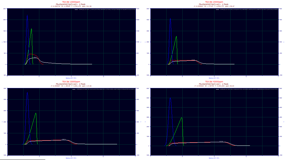
The blue curve is the deconvolved Gaussian, the peak the model predicts if there was no IRF and no concentration-dependent a3 chromatographic distortion.
The a1 location values, the mean of this underlying Gaussian, are again close to identical in all four data sets and occur at the sharp discontinuity in the rise of the IRF-deconvolved shape in red.
Concentration and a2
As you will note, the deconvolved Gaussian widths (evident in the blue Gaussian and green HVL peaks) increase with concentration. There is some support for the premise.
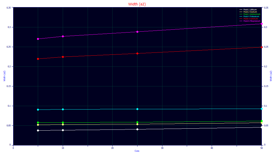
In fitting analytic peaks, we have observed an increase in a2 with an increase in analytic concentrations. The above plot is for GenHVL<ge> fits of the cation data that was used in the second IC tutorial. The increase is a2 appears to track the magnitude of the a3 distortion. The a3 distortion is greatest in magnitude in the Ca+ (red) and Mg+ (magenta) peaks and those do show an increase in a2 with concentration. The K+ peaks (cyan) have very little a3 distortion, and they are close to constant in a2 across concentration.
In these far higher concentration GenHVL[Yp2] overload fits (10000-40000 ppm vs. 5-50 ppm for the analytic fits), the increase in a2 is 4.7% from 1% to 2% concentration, 44% from 1% to 3% concentration, and 86% from 1% to 4% concentration. Since we are generating model-dependent deconvolutions, we do not know if the a2 would actually increase in this way. To test such, we would need a column/detector capable of producing the green peaks instead of the white overload shapes at these high concentrations. We can thus only note that there is evidence of a2 increasing with concentration at analytic concentrations when there is significant fronting or tailing.
Click OK to close the Review, click OK to accept the default name for the fit, and click OK to confirm. Click OK once more to return to the main screen.
The Simpler Overload Models
The GenHVL[YpE] model is the simplification of the GenHVL[Yp] with the decay power fixed at 1.0, a Laplace zero-distortion density. As we saw in the first set of fits, the power of decay=1 tails generally apply to overload peaks with a full envelope (a linear region between the rise and decay). For such full envelope shapes you may wish to fit the GenHVL[YpE] model. The GenHVL[YpE] and GenHVL[Yp] fits will be nearly identical for the three full envelope overload shapes. It is only with the first data set lacking such an envelope where there is a significant difference in the goodness of fit and parameter values. If you are interested, you can also use the ZDD dialog to lock the [Yp] power (kurtosis adjust) at 1.0, and you will see the same results as the GenHVL[YpE] fit. Although closed form models fit very quickly, the simpler GenHVL[YpE] is much faster than the GenHVL[Yp]. If you choose to fit the GenHVL[YpE] model, you should see 362.4 ppm for the unaccounted variance of the first fit.
The GenHVL[Yp2E] model is similarly the simplification of the GenHVL[Yp2] with this decay power fixed at this 1.0 exponential decay. This model must also be limited to full envelope fits. Because this model forces a 1.0 power of decay dilation in fits where a5 fit slightly above 1.0 as the envelope broadened, certain of the GenHVL[Yp2E] fits will be somewhat weaker. As with the GenHVL[Yp] model, one less parameter is fitted, and the fits will be significantly faster.


 |